Introduction
The goal of this project was to explore DSP algorithms gradually and, as a final result, to implement a band-pass filter that adjusts its passband so that only the dominant frequency of a signal can pass through. The algorithms were applied to vibration data measured by an ADXL345 accelerometer mounted on a real vibrating object - a kitchen mixer running at different speed levels.
System architecture
General system architecture
DSP pipeline
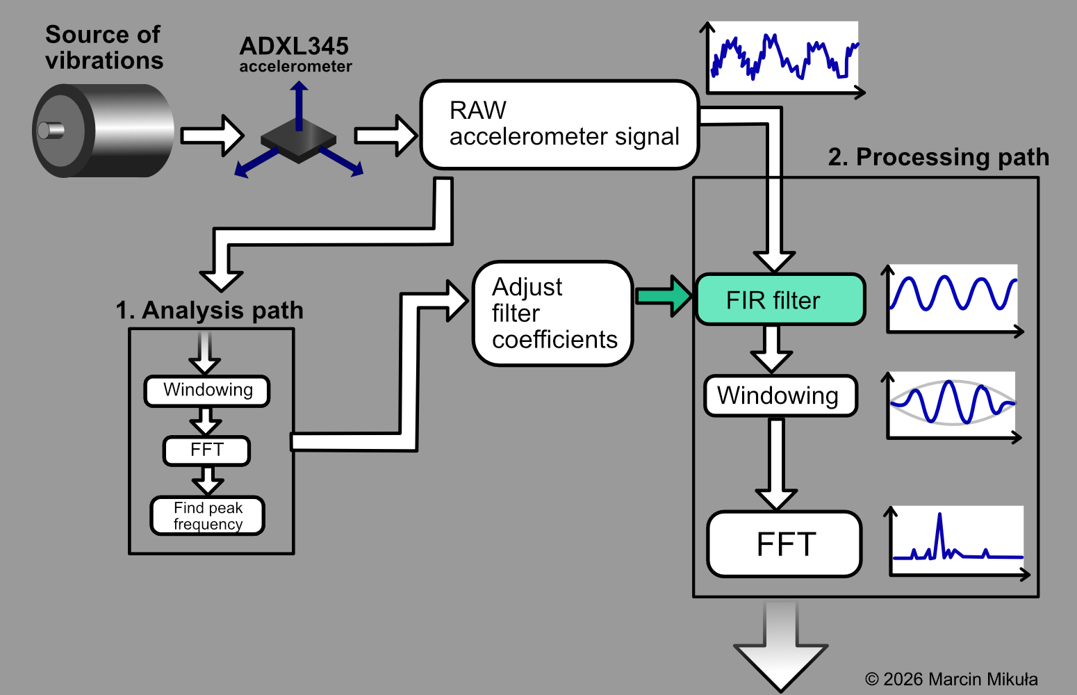
DSP pipeline overview: raw accelerometer data flows through the analysis path (FFT + peak detection) and the FIR filter processing path.
The measured object produces vibration, which is measured by an ADXL345 accelerometer. Only data from one axis (X) is processed, due to the system's RAM memory constraints.
- Once the raw signal is acquired, the analysis path begins by locating the peak frequency. A chunk of the signal is multiplied by Hann window, and the Fast Fourier Transform is then computed. From the resulting spectrum, the dominant frequency is identified and the corresponding FIR filter coefficient set is selected.
- Then the raw signal is filtered by a bandpass FIR filter with adjusted coefficients. Hann window is applied and then FFT is computed. The processed output is sent to PC with UART.
FreeRTOS tasks
The system operation was split into a few tasks that are supervised by the FreeRTOS operating system.
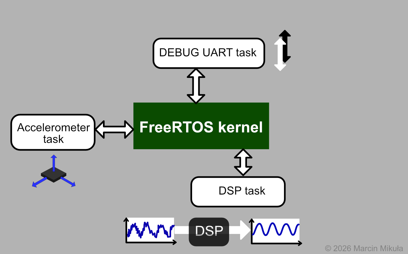
FreeRTOS tasks and their interactions.
There are three main tasks in the project:
- Accelerometer task - initializes, configures, and reads raw data from the accelerometer. It coordinates reading from the ADXL345 FIFO buffer via SPI interface using the DMA mechanism. Then the task sends the message to the DSP task via a message queue.
- DSP task (Digital Signal Processing) - adjusts filter coefficients, applies FIR filter and windowing, computes FFT, and sends the data via message queue to the UART task.
- An additional feature is that the FIR filter is applied as the button is pressed, to see and compare the on/off results.
- DEBUG UART task - responsible for transmitting the data to a PC computer, where the data is saved and visualized.
- Heartbeat task - toggles the built-in LED2 diode to indicate continuous, uninterrupted operation of the system. It is a remnant from the system debugging stage, when it was not optimized and the task scheduling was hard to observe.
ADXL345 accelerometer
MEMS accelerometers - how they work?
Micro Electro Mechanical Systems (MEMS) are small mechanical structures of microscopic size, coupled with microelectronic circuits. They may be used to design small actuators or precise sensors with a very small footprint.
There are a few types of MEMS, depending on their application:
- Piezoresistive - they are able to sense mechanical deformation (strain gauges)
- Capacitive - linear acceleration (accelerometers)
- Gyroscopic - angular rate (gyroscopes)
ADXL345 is one of the MEMS accelerometers that uses a differential capacitance mechanism, explained in the diagram below.
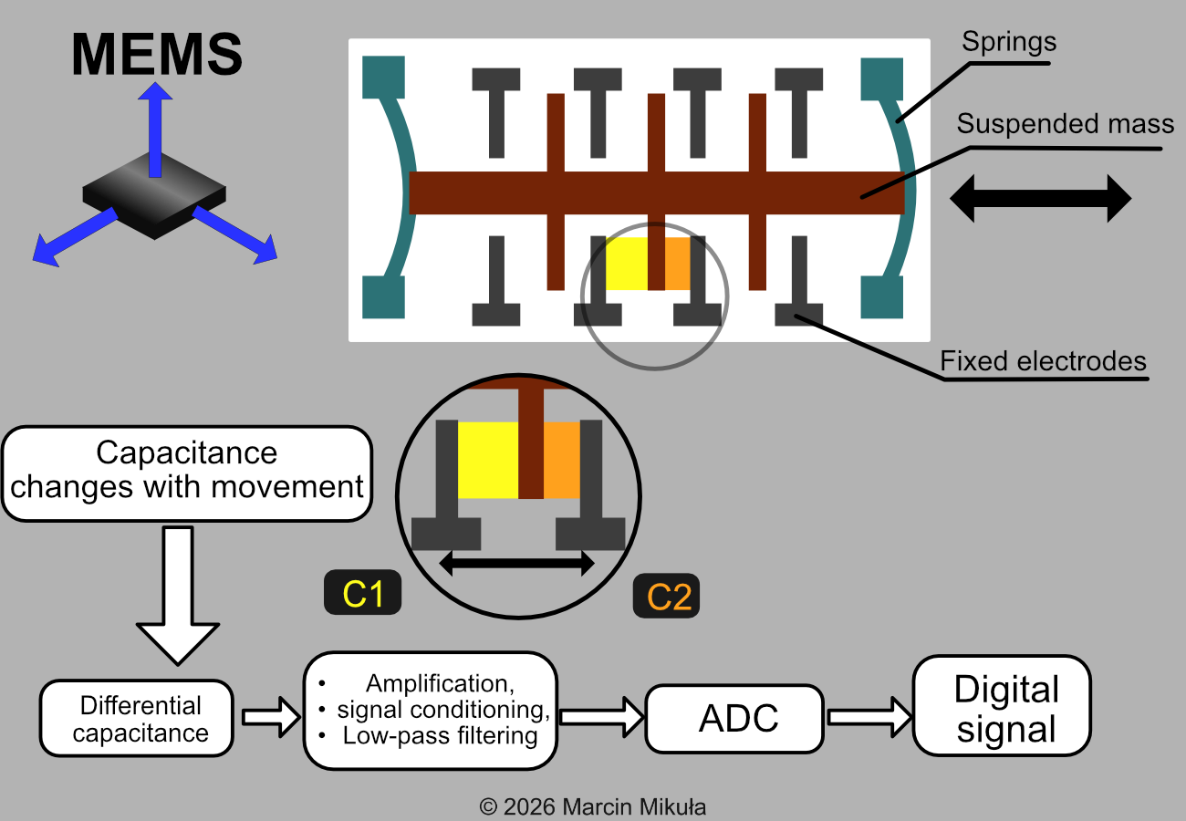
A diagram explaining how the MEMS accelerometer is built and how it works. A mass is suspended on polysilicon springs and moves when acceleration occurs in a certain direction. That results in a change in capacitance between the suspended mass and the fixed electrodes.
ADXL345 accelerometer features and limitations:
- Up to 3200 Hz ODR (output data rate) - adjustable: 3200, 1600, 800, 400... Hz
- 32-sample FIFO buffer
- I2C and SPI communication interfaces
According to the datasheet, ODR greater than 800 Hz requires the use of SPI, and a custom timing procedure when retrieving data from the FIFO buffer.
Why SPI was chosen
The 3200 Hz and 1600 Hz output data rates are only recommended when SPI is clocked at 2 MHz or higher, so SPI was the natural choice for keeping the higher data rates within reach. I2C, though more convenient to wire up, has a maximum clock of 400 kHz in standard mode, which falls well short of what is needed for the higher ODRs.
Why 800 Hz ODR was chosen, and the tradeoffs
Reading from the FIFO carries a timing constraint: according to the datasheet, at least 5 µs must elapse after the data registers are read before the next entry is popped into the DATAX, DATAY, and DATAZ registers. At 3200 Hz ODR this constraint is tight enough that the read loop must include an explicit delay, which ties up the CPU during every FIFO read.
This is what drives the decision at which ODR to operate. The higher ODRs would require at least a 2 MHz SPI clock, which in turn would require implementing that explicit inter-read delay mechanism. In practice, this means the DMA transfer finishes but the CPU has to spin-wait for the 5 µs gap before starting the next byte.
There were also practical reasons to stay at 800 Hz. The DSP algorithms consume both time and memory, and raising the sample rate could have destabilized the system, particularly as it runs on an STM32 with limited RAM. For these reasons, 800 Hz was selected as the operating output data rate.
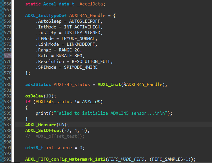
ADXL345 accelerometer software configuration.
The use of FIFO buffer
A FIFO buffer helps offload the main processor, because it can read the data in batches instead of reading sample by sample.
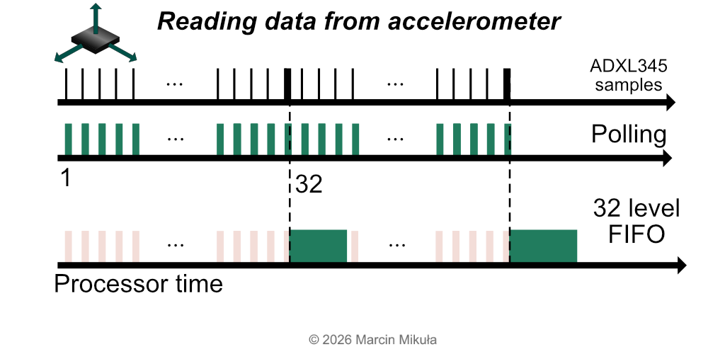
FIFO vs Polling. Overall processor time usage is shorter when using FIFO.
Usually, when reading data from sensors, a polling mechanism is used. The microcontroller checks if sensor data is ready and then reads from the device, repeating at every time interval.
A better method uses interrupts and a FIFO buffer. The internal sensor buffer stores samples, and once the number of samples equals the FIFO level that was set (could be 32, 16, 8... samples), an interrupt is triggered. The microcontroller wakes up, reads all stored samples at once, and goes back to other work.
Reading with DMA
What is more interesting, this can also be done not by the microcontroller itself, but with a DMA (Direct Memory Access) controller. This works like a helpful coworker that runs a simple particular task in parallel with the main processor. In this project, reading with the SPI interface using DMA was used. The ADXL345 accelerometer measures the vibrations and puts data into the FIFO buffer. After the FIFO is full, the interrupt from the ADXL345 appears and the DMA reads the samples directly into RAM, without occupying the CPU.
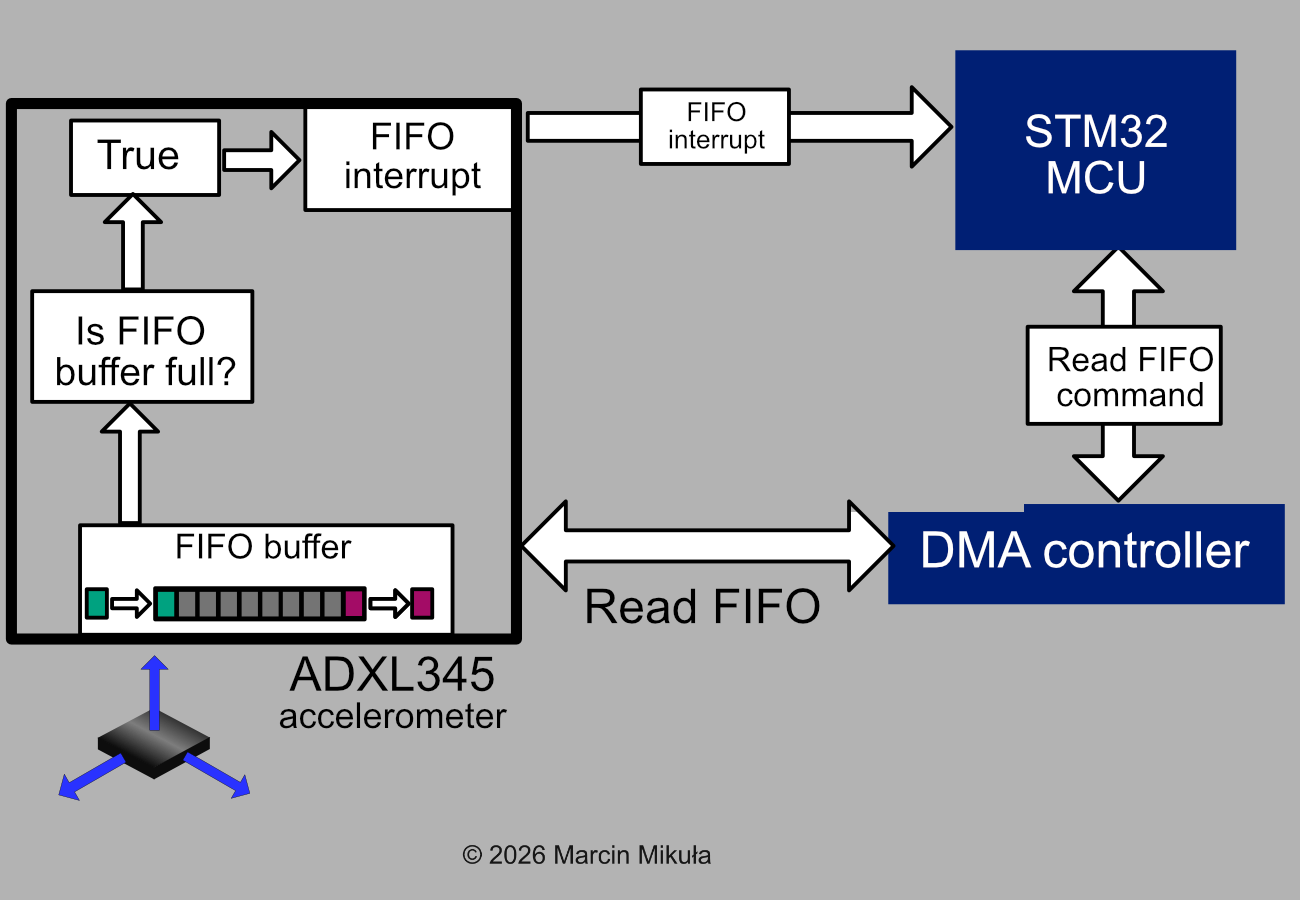
Retrieving data from FIFO with DMA controller.
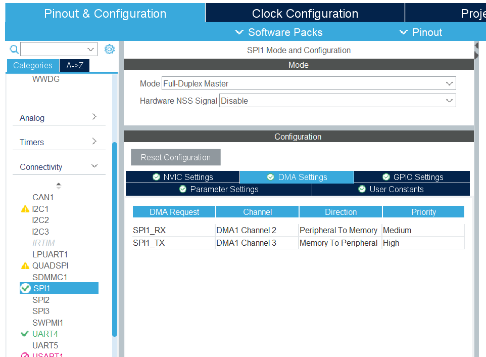
Configuration of SPI communication DMA requests in STM32CubeIDE.
Embedded Digital Signal Processing
CMSIS DSP library
CMSIS (Common Microcontroller Software Interface Standard) is an open-source set of reusable tools and APIs that help simplify development of new applications in embedded systems. These are aimed at ARM Cortex-M based microcontrollers and are provided by ARM Holdings.
Its components include, but are not limited to, Neural Networks, RTOS, Driver, and DSP libraries. In this project I used the CMSIS DSP software library, as it provides common signal processing functions such as FFT, FIR filter, and others optimized for ARM Cortex-M processors.
Fast Fourier Transform (FFT)
The Fast Fourier Transform is an algorithm that converts a signal in the time domain to its representation in the frequency domain. It can also work in reverse - the signal can be restored from its spectrum with the Inverse FFT.
Worth mentioning: the more N samples the FFT is calculated from, the better the frequency resolution is. There is my article on FFT where a reader will find more information on the topic: lowentropy.pl/articles/dsp/fft_explained/
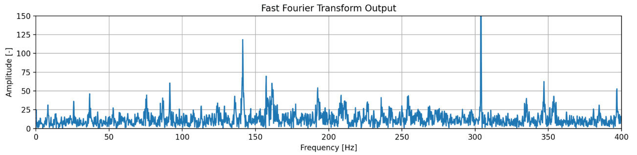
FFT frequency spectrum calculated with N=4096 samples.
Short-Time Fourier Transform (STFT)
STFT is a way to analyze how the signal frequency spectrum changes over time. In its basic form, a signal is divided into shorter segments of equal length and then FFT is computed separately on each segment. The results are plotted next to each other, forming a 2D spectrogram where the horizontal axis is time, the vertical axis is frequency, and the color intensity represents amplitude.
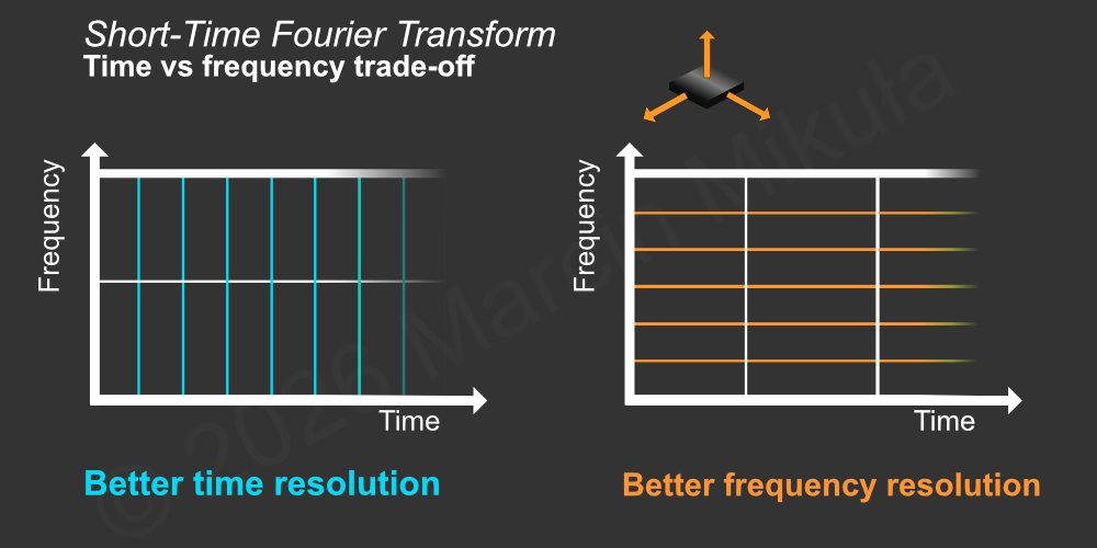
Comparison of STFT spectrograms computed with N=128 and N=1024 samples, illustrating the time vs. frequency resolution tradeoff.
In this project, since it was aimed to work in real-time and the whole signal is not available, the FFT is computed per segment and spectrograms are plotted after each other over time.
There is a tradeoff between frequency and time resolution. While a larger number of samples (N) provides better FFT spectrum resolution, it takes longer to record those samples. On the other hand, a smaller N gives a faster update rate but a coarser frequency spectrum - individual frequency bins are wider, so nearby peaks can be harder to distinguish.
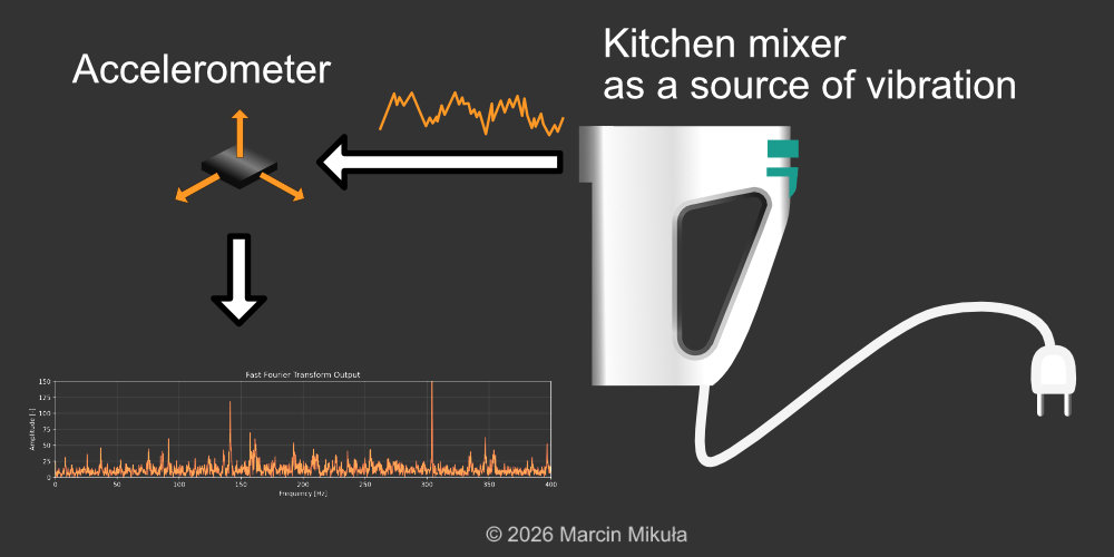
Kitchen mixer - the source of vibrations used for measurements. It runs at different, fixed, and stable speeds, producing a signal with a dominant frequency that can be changed.
This was shown with real data recorded from the kitchen mixer, whose speed was gradually changed. N = 128 and N = 1024 are compared. Note that although the small N gives a rougher spectrum, it is able to capture the electric motor dynamics, while at N=1024 the transitions are harder to see because each frame takes longer to record.
Another concern is that because it takes longer to capture the signal batches, the system runs at a lower FPS rate, which can matter in real-time monitoring systems.
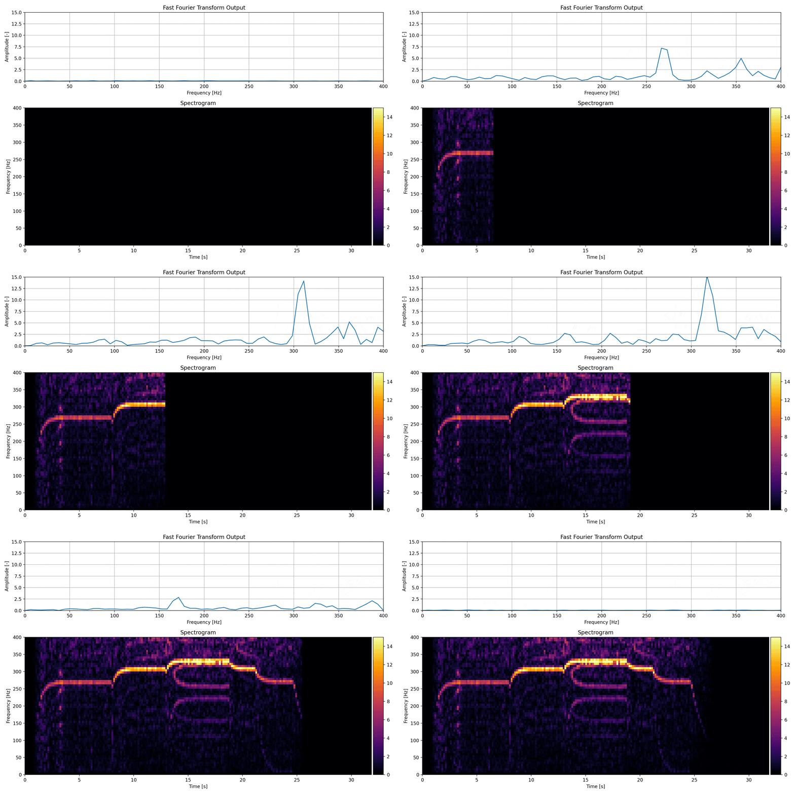
Spectrogram of a kitchen mixer signal computed by STFT with N = 128 samples.
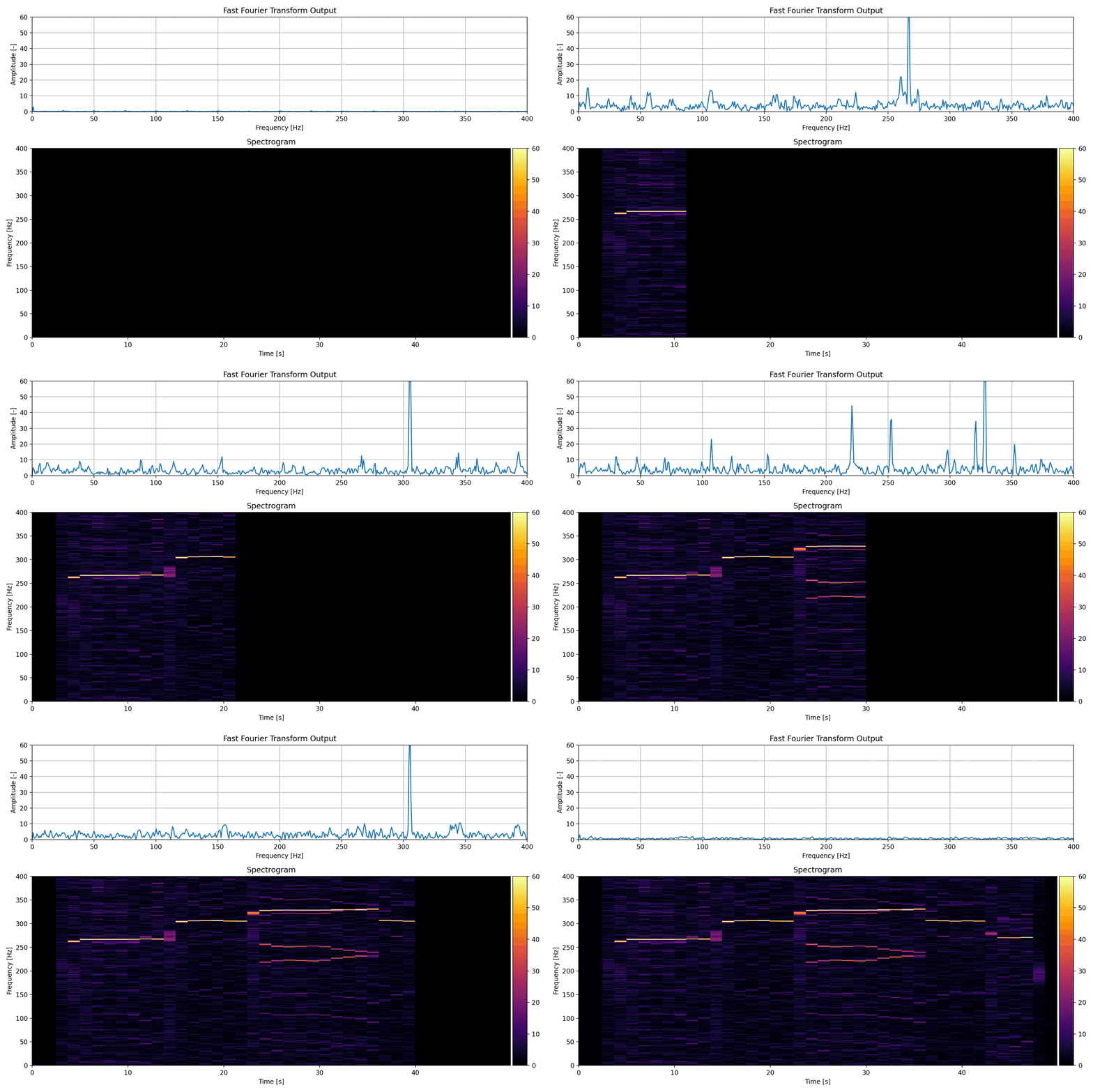
Spectrogram of a kitchen mixer signal computed by STFT with N = 1024 samples.
Windowing
In previous sections, windowing was mentioned. It is one of the basic DSP preprocessing functions and helps to reduce spectral leakage and emphasize the correct peak frequency. I wrote about it in more detail in my article on spectral leakage: lowentropy.pl/articles/dsp/digital_filters_explained/
Why Hann window?
Often in literature the Hanning (Hann) window is mentioned as a commonly used window type suitable for most applications. It attenuates the ends of the signal batch so that any discontinuities have minimal effect on the spectrum. The equation for the Hann window is:
where:
- w(n) - value of window element
- n - current element index
- N - last window vector index; N+1 is window length
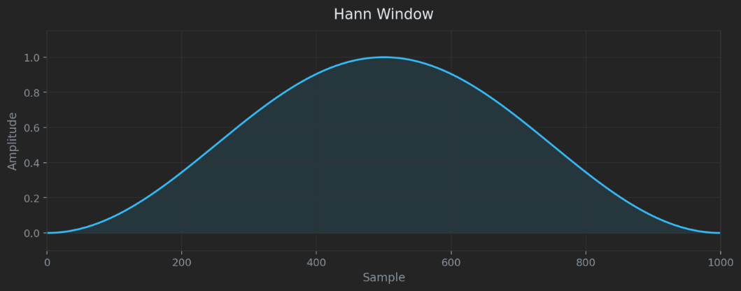
Hann window shape - amplitude tapers smoothly to zero at both ends.
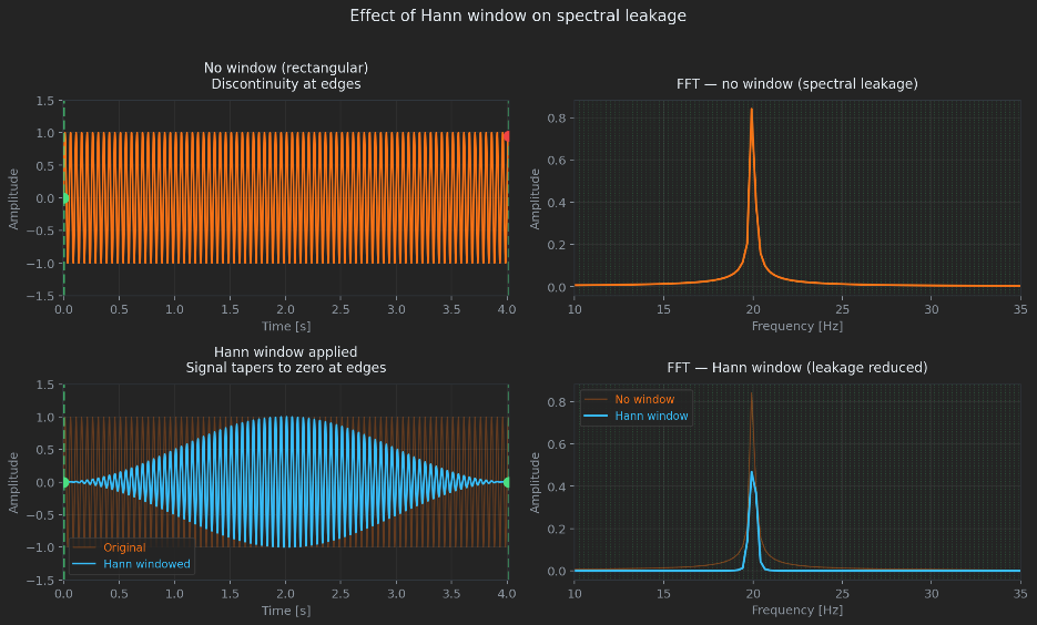
The effect of applying a Hann window on a signal frequency spectrum. Although the peak amplitude is slightly smaller, the spectral leakage is significantly reduced.
Below are examples of how Hann windowing looks in a real system - pictures of the FFT spectrum and spectrogram showing how it changes over time. When the button was pressed, the window was applied before FFT. As is clearly visible, the overall noise and spectral leakage were reduced.
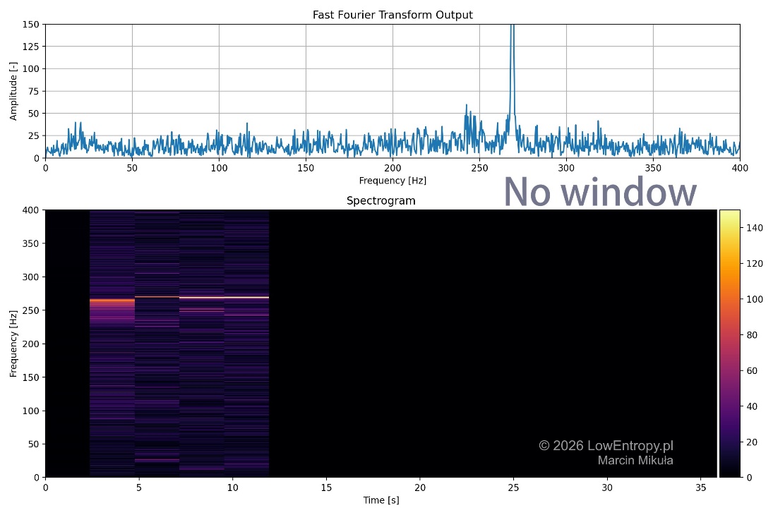
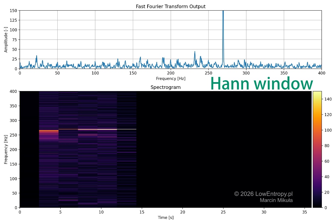
An example of Hann windowing - reduced spectral leakage. Left: no window applied. Right: Hann window applied.
FIR filters
Finite Impulse Response (FIR) filters are digital filters that use only current and past inputs. In this project a bandpass filter was used so that the interesting part of the frequency spectrum is kept unattenuated while everything outside the passband is suppressed.
I wrote an article about Digital Filters where I described FIR and IIR filters in more detail: lowentropy.pl/articles/dsp/digital_filters_explained/
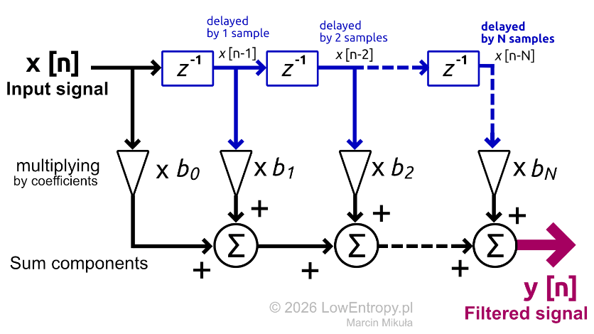
FIR filter structure: delayed input samples are multiplied by coefficients and then summed.
As mentioned in the article above, the more coefficients, the better the result. This was shown in the GIF below, where the signal consists of two sine waves of low and high frequencies. A FIR kernel with fewer coefficients has a less sharp frequency cutoff.
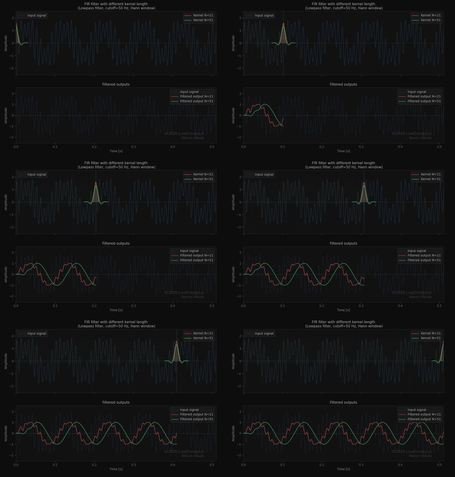
Two FIR filters with different kernel lengths applied to the same signal in real time.
The longer the kernel, the more FIR coefficients are needed. I decided to limit N to 201, because increasing the number of coefficients beyond this does not offer noticeably better results while requiring more RAM memory.
An example of how FIR works in a real system is shown below - real data from the ADXL345, with the band-pass FIR filter toggled on and off with a button. Note that the spectrogram looks much cleaner with the filter on.
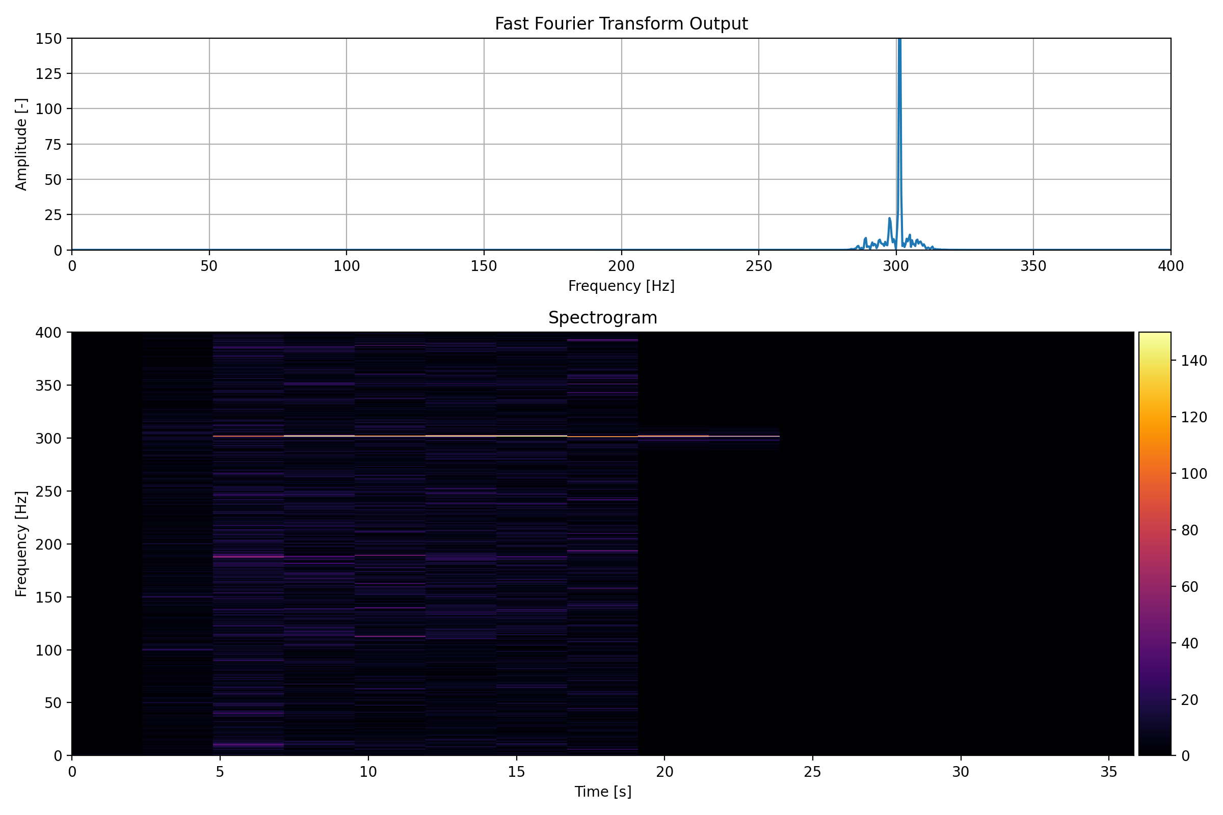
Band-pass FIR filter toggled on/off in real time with a button.
Implementation
Setup and wiring
Kitchen mixer as a source of vibrations
As mentioned before, the experiments were conducted with a real vibrating object. The main idea was to produce a signal with a changing dominant frequency that would have some noise in it. Funnily enough, a kitchen mixer turned out to be a good candidate for this - it can run at different, fixed, and stable speeds, and apart from that, it has some noise so it is not a clean, pure sine wave.
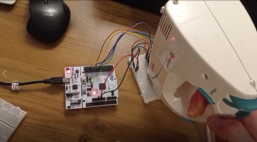
Kitchen mixer as a source of vibrations. The main advantage of the device is that it can run at different, fixed, and stable speeds. It has some inherent noise, making it a more realistic test signal than a pure sine wave.
Wiring
This project required proper wiring to the ADXL345 accelerometer sensor. The SPI interface was chosen and, because FIFO was used, it required an extra connection to the STM32 Nucleo board for the interrupt pin. The accelerometer was placed directly on the mixer housing to pick up the vibrations.
Embedded Software Implementation of DSP algorithms
Windowing


Function that initializes a Hann window as a set of numbers. A vector of given length is created.
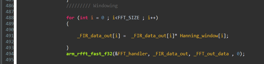
Applying a window means multiplying element-wise the window vector and the signal buffer.
FFT
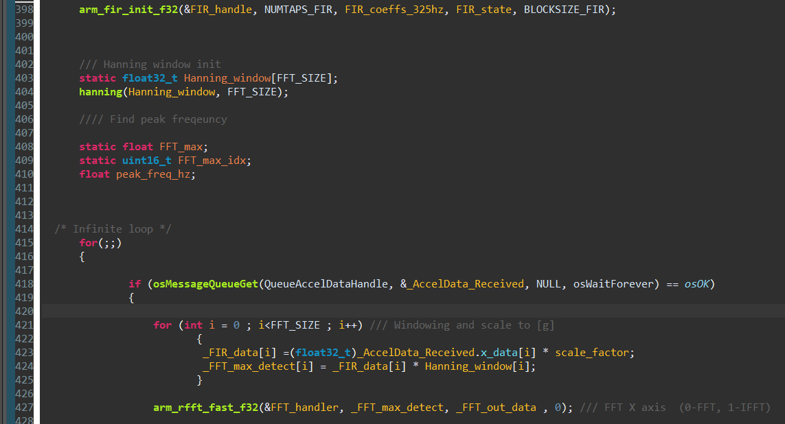
After scaling raw data to [g] units and windowing, the arm_rfft_fast_f32 function is executed. Because the output contains both real and imaginary numbers, the result is recalculated into amplitude values.
Filter coefficients
The FIR coefficient sets are pre-calculated and stored in the STM32 MCU's memory. They were generated using the FIR filter design tool from Virtual Labs, IIT Kharagpur, which provides a straightforward interface for specifying the filter type, passband frequencies, and number of taps.
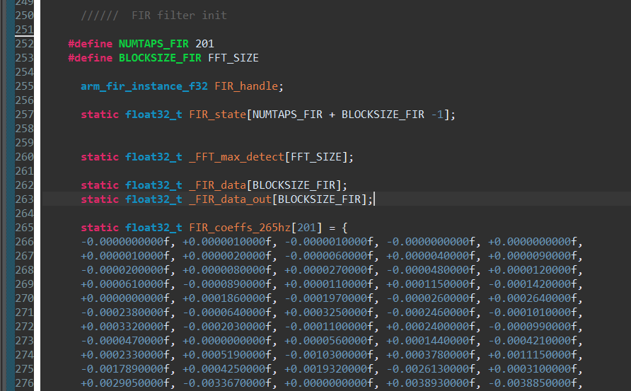
FIR filter coefficients for 265 Hz frequency.
Mechanism behind changing FIR filter coefficients
The kitchen mixer has only 5 speed levels and three of them were used. The main purpose was to test the algorithm, so the device was not under load. After some experiments and frequency spectrum analysis it turned out that the mixer only produces vibrations at the following frequencies, depending on speed level:
- 265 Hz (speed 1)
- 300 Hz (speed 2)
- 325 Hz (speed 3)
Filters were designed with a bandwidth of about 20 Hz. If the dominant frequency fits into the desired range, then the FIR filter coefficients are adjusted accordingly.
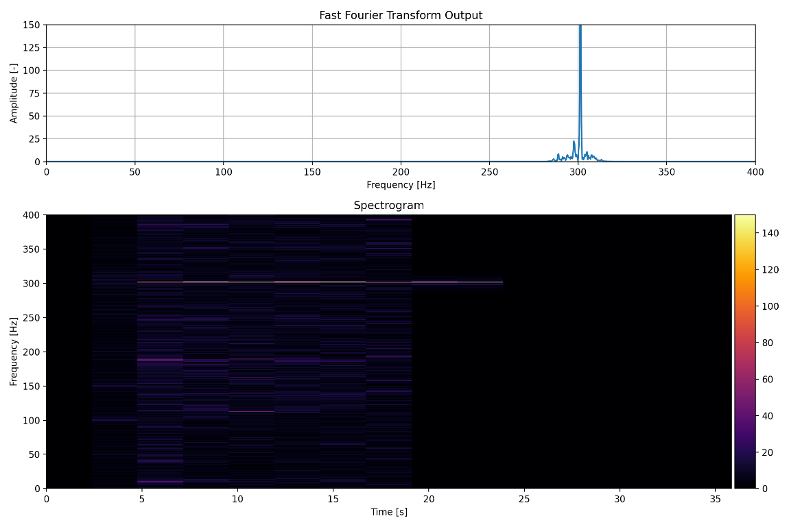
Bandpass filter operation for 300 Hz frequency (bandwidth of 290 - 310 Hz).
DMA usage for ADXL345 reading
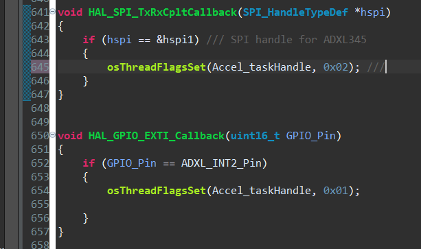
Interrupt Service Routines of SPI communication and External interrupts with GPIO pins. Thread flags are set so that FreeRTOS can use this mechanism to synchronize its tasks.
Configuration in STM32CubeIDE:

Fragment of NVIC (Nested Vector Interrupt Controller) list. External interrupts and DMA interrupts are allowed.
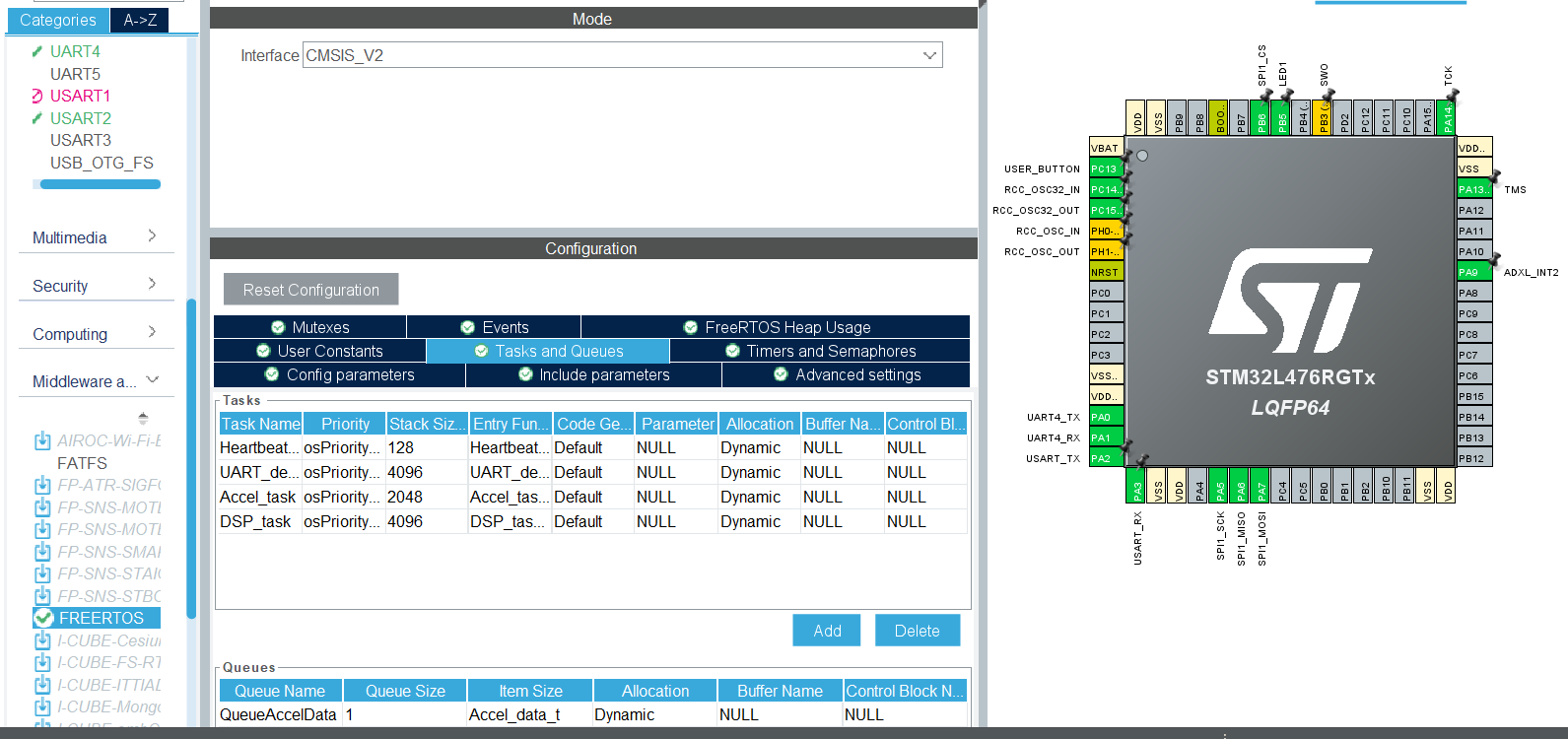
CMSIS V2 FreeRTOS tasks list in STM32CubeIDE.
Demonstration
Windowing on/off
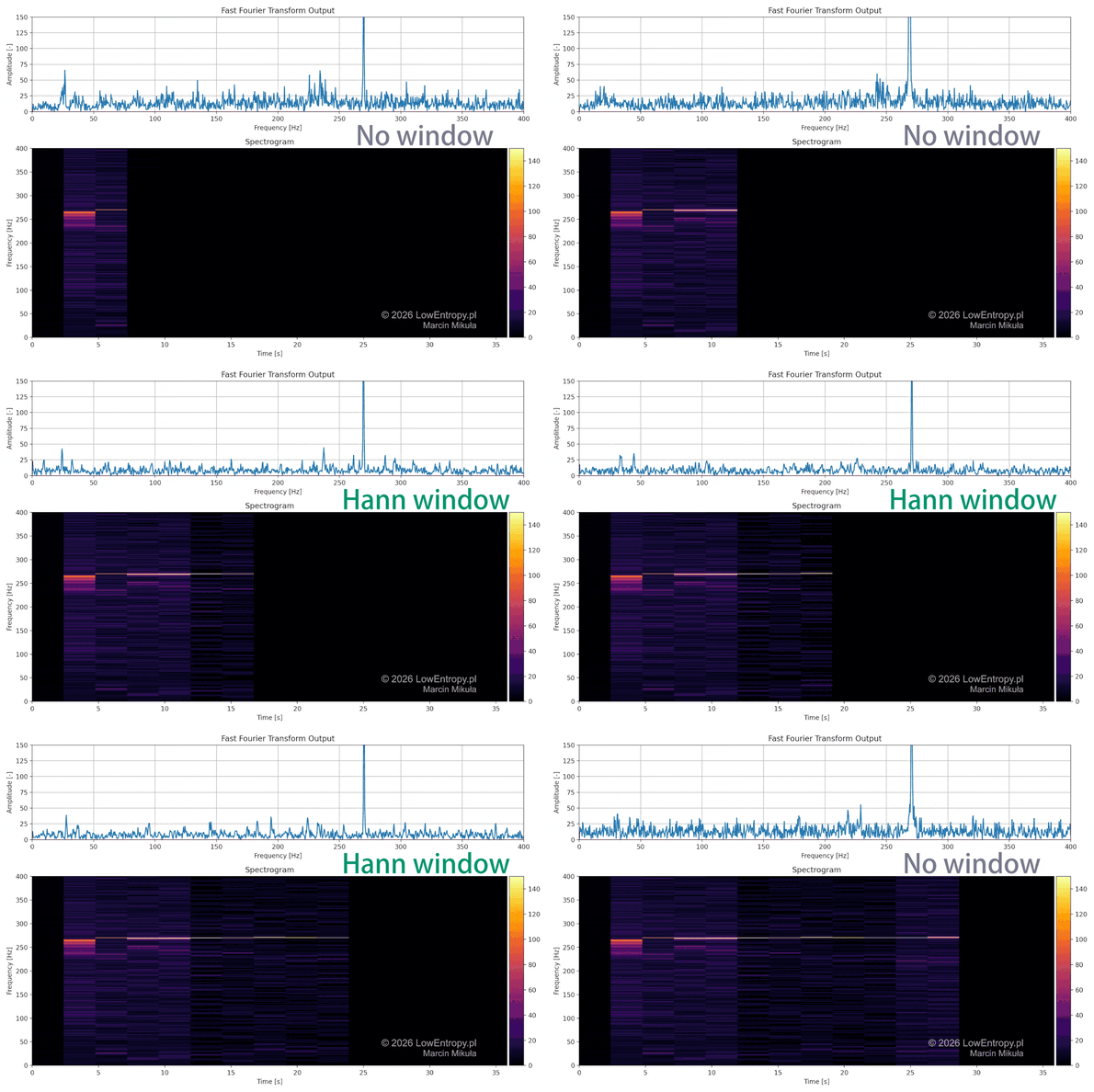
Windowing applied and removed in real time - the effect on spectral leakage is clearly visible.
FFT with different number of samples N
Shown below with different number of samples (128, 1024, 4096):
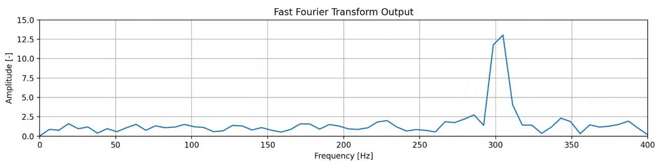
FFT spectrum with N = 128 samples - broad peak, lower frequency resolution.
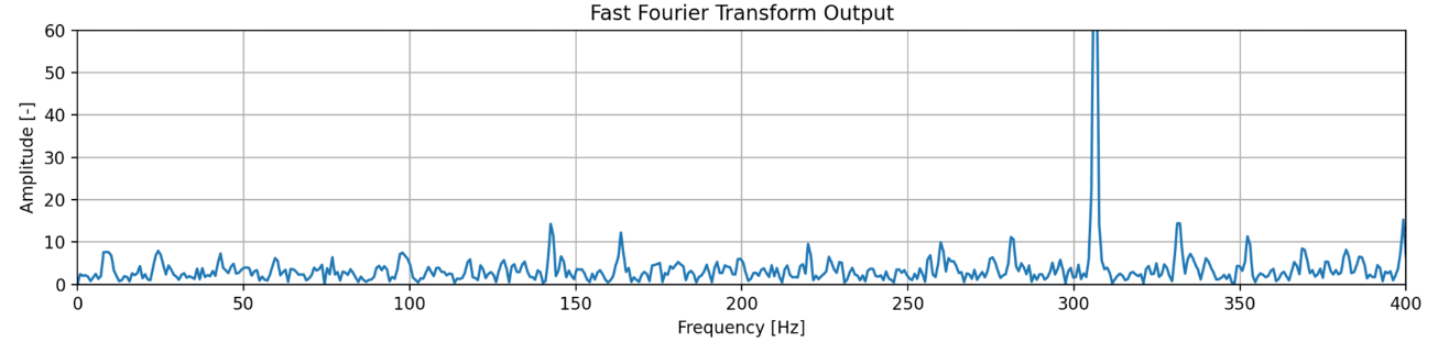
FFT spectrum with N = 1024 samples - sharper peak, better frequency resolution.
FFT spectrum with N = 4096 samples - highest frequency resolution.
Spectrogram with different number of samples - time vs frequency resolution tradeoff in practice
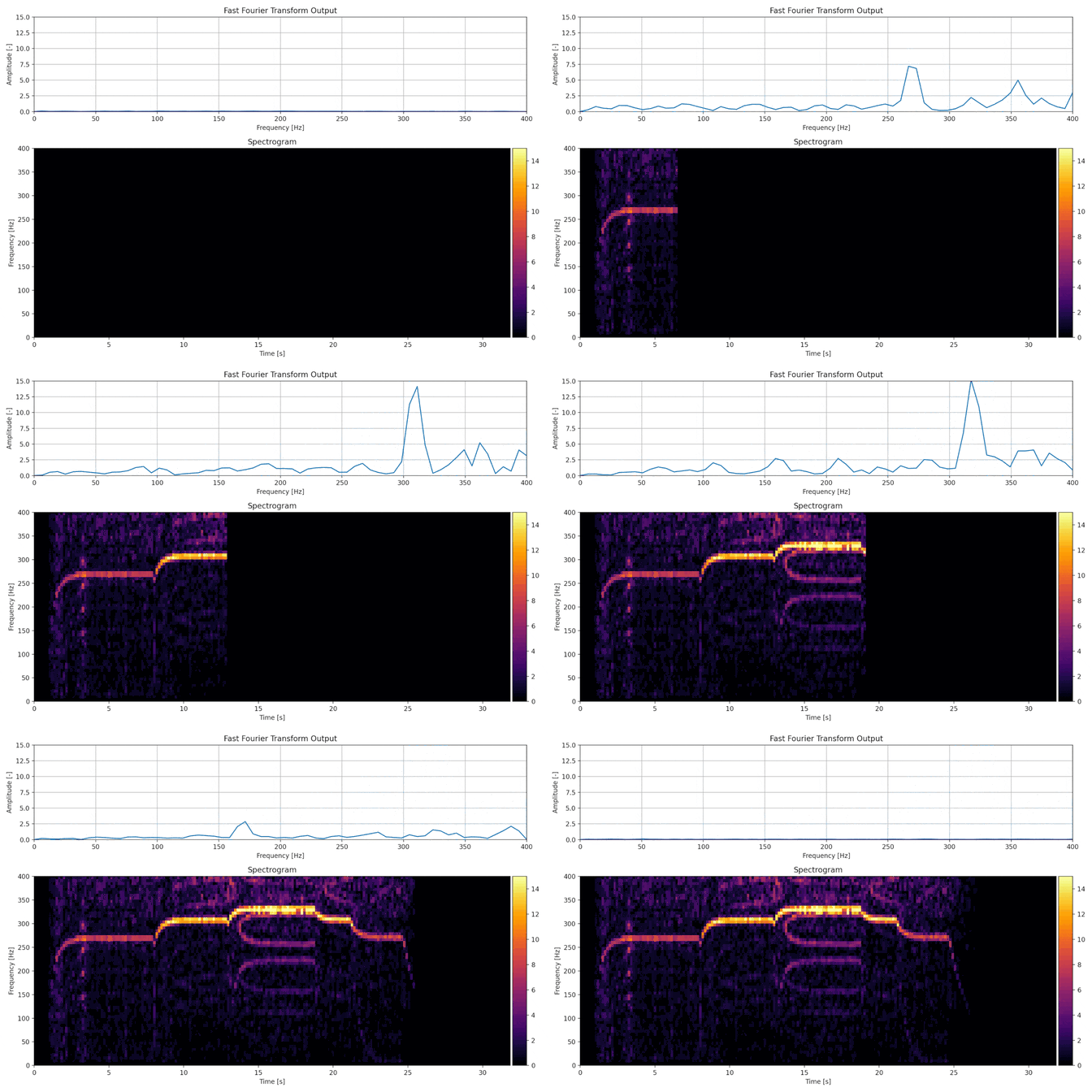
Spectrogram of a kitchen mixer signal computed by STFT with N = 128 samples.
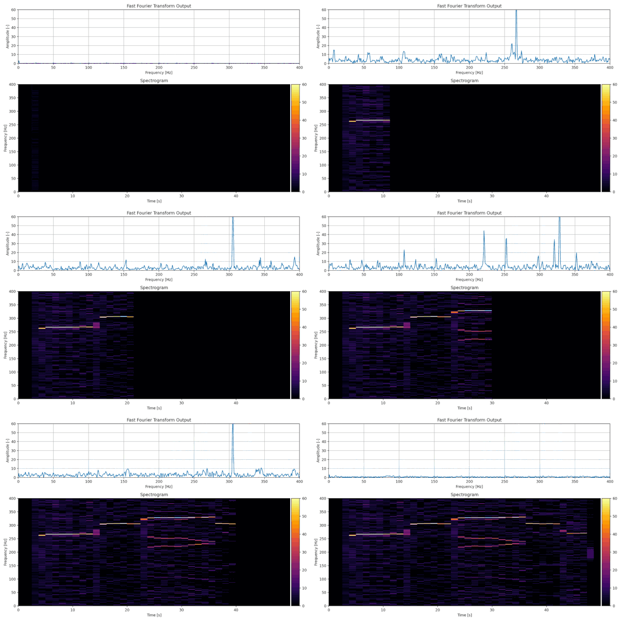
Spectrogram of a kitchen mixer signal computed by STFT with N = 1024 samples.
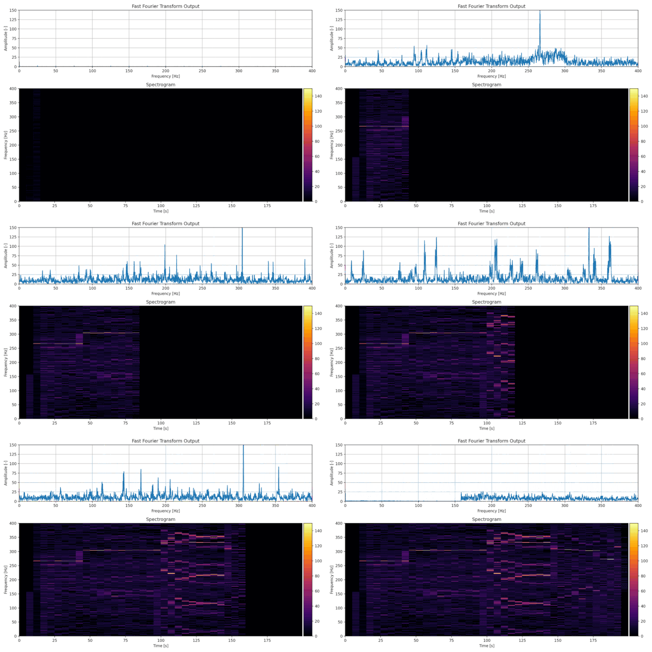
Spectrogram of a kitchen mixer signal computed by STFT with N = 4096 samples.
GIF - final result
Demo GIF will be added here.
Future work
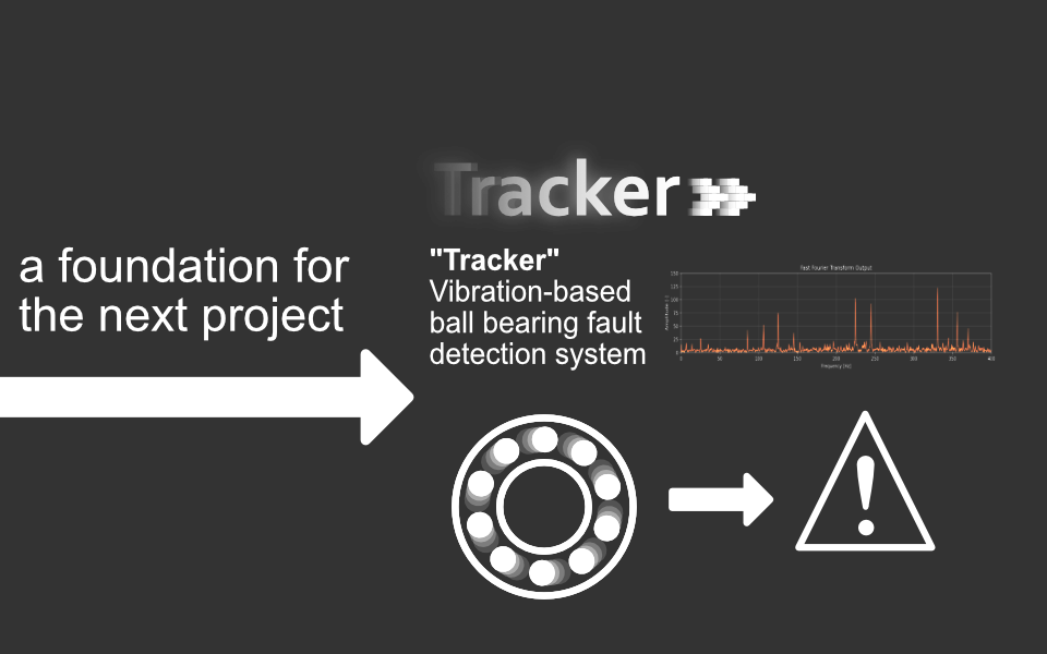
This project lays the groundwork for a more capable condition-monitoring system. The planned next step is built around the IIS3DWB accelerometer and the STM32N6 microcontroller. The IIS3DWB offers a flat frequency response up to 6 kHz and a sample rate of 26.7 kHz, which is a significant step up from the ADXL345's 800 Hz ODR used here.
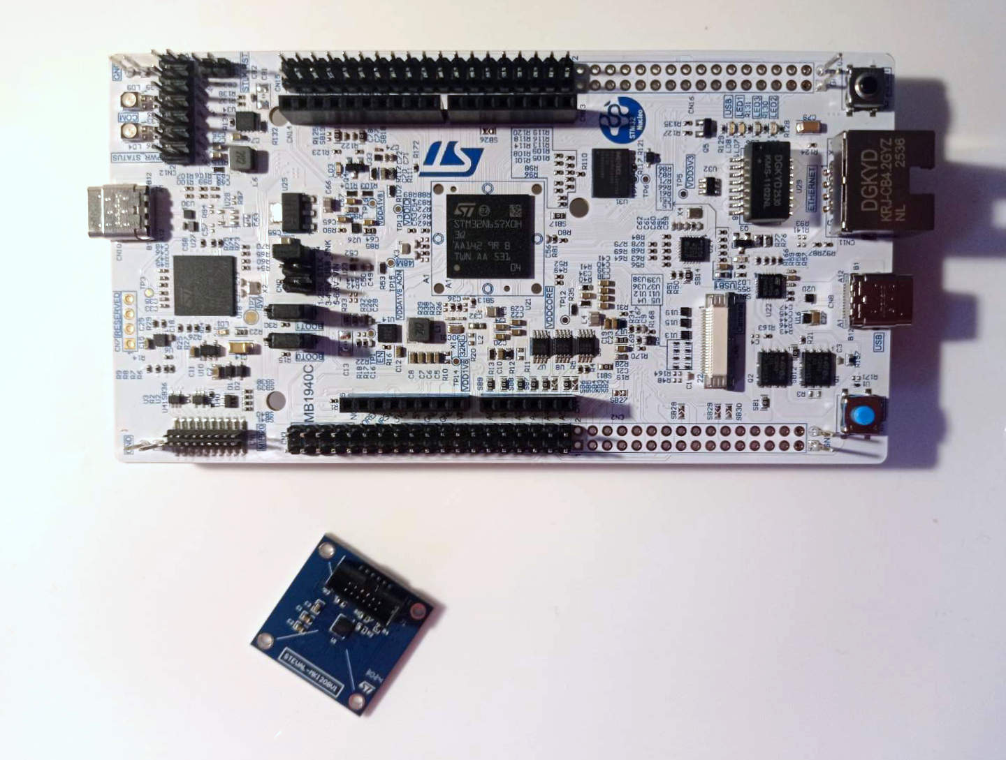
The hardware that will be used in the next project.
The goal is to detect ball bearing faults at an early stage and use that information for predictive maintenance, to estimate when a failure is likely to happen. Then the downtime can be planned in advance rather than responding to an unexpected failure. This is most valuable in machines that are difficult to service or cannot easily be stopped, where anticipating a failure is far more useful than reacting to one. The system would apply machine-learning algorithms to classify the bearing condition from the vibration signal.