FFT Explained

In most real-world situations you cannot tell just by looking at a raw signal what frequencies are inside it. A time-domain waveform shows how amplitude changes over time — but gives no direct information about frequency content. The Fast Fourier Transform (FFT) solves this: it converts a time-domain signal into its frequency-domain representation, revealing exactly which frequencies are present and at what amplitudes.

FFT is an efficient algorithm for computing the DFT (Discrete Fourier Transform). Where a naive DFT requires O(N²) operations, FFT achieves the same result in O(N log N) — making it fast enough for real-time processing in embedded systems and large-scale data analysis alike.

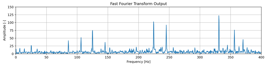
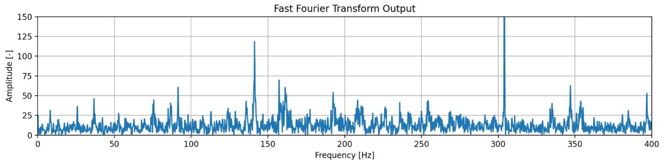
An example FFT output — frequency on the x-axis, amplitude on the y-axis.

How the algorithm works

FFT decomposes a time-domain signal into the set of frequencies it is made of. Technically it produces both real and imaginary parts, but in practice we work with the magnitude spectrum — how much of each frequency is present in the signal.

The simplest way to build intuition is to start with a clean sine wave. Consider a signal at a single frequency — 20 Hz. Sampled over a few seconds and viewed in the time domain, it looks like this:

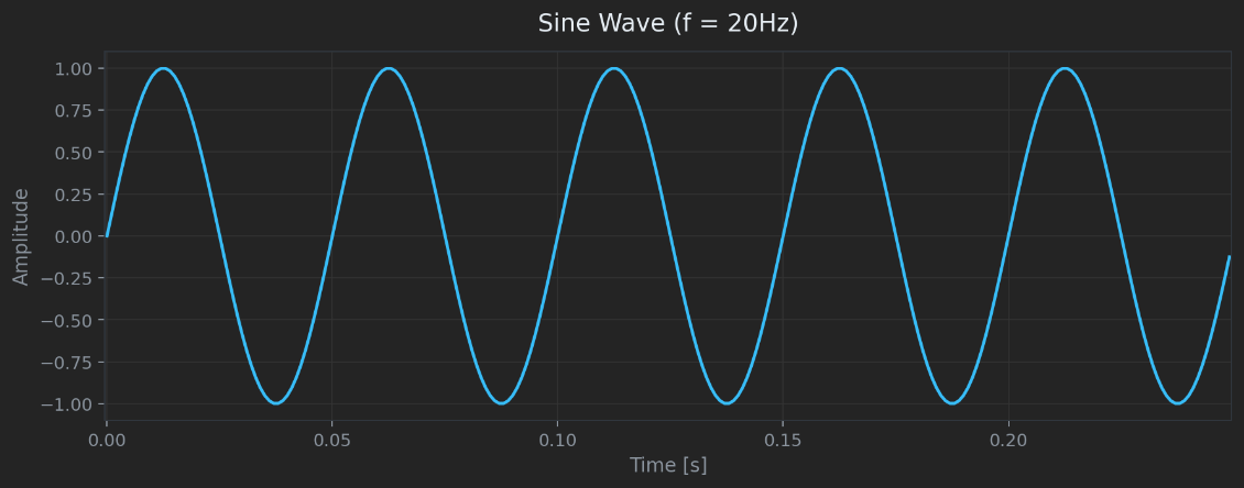
A pure 20 Hz sine wave sampled over time.

After applying the FFT algorithm, the output spectrum shows a single sharp peak at exactly 20 Hz — and nothing else. One frequency in, one peak out.

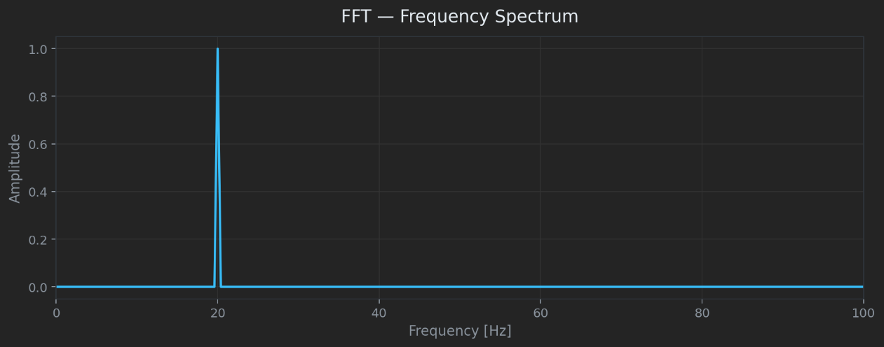
FFT output of the 20 Hz sine wave — a single peak at the signal's frequency.

Now consider three sine waves of different frequencies added together to form a composite signal. In the time domain the waveform looks complex and hard to interpret:

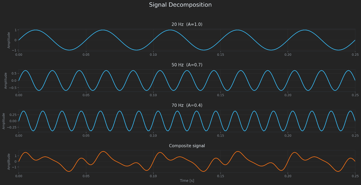
A composite signal built from three sine waves of different frequencies and amplitudes.

The FFT immediately reveals the structure — three peaks, each at one of the component frequencies, with amplitudes proportional to the component's strength in the signal:

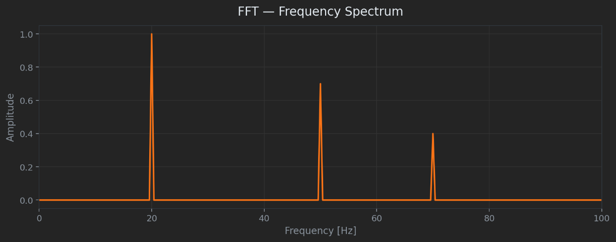
FFT output showing three peaks — one for each frequency component in the composite signal.

This is the core purpose of FFT: it lets you look at a signal in the frequency domain and see its components — even when those components are completely invisible in the time domain.

Noise and other signal components

DC component

If a signal has a non-zero mean value — a constant offset — the FFT will produce a peak at 0 Hz. This is called the DC component. It is typically removed before further analysis, as it can dominate the spectrum and obscure the signal components of interest.

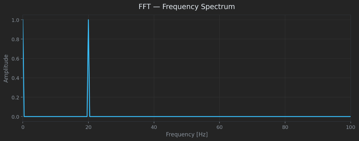
A DC offset in the signal produces a large peak at 0 Hz in the FFT output.

Noise impact

Adding Gaussian noise to a signal distributes energy across all frequencies, raising the noise floor across the entire spectrum. When the noise amplitude is low, the signal components remain clearly visible above it. When the noise is strong enough to exceed the amplitude of a component, that component may be buried and impossible to detect.

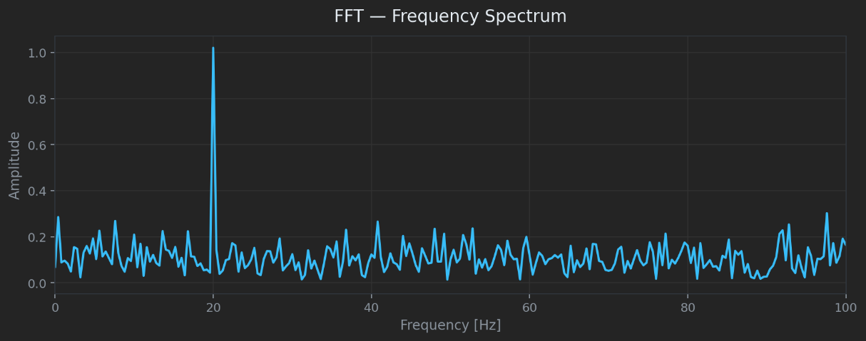
Gaussian noise raises the noise floor across the entire spectrum. High SNR components stay visible; weak ones can disappear.

The ratio of signal power to noise power is called the Signal-to-Noise Ratio (SNR). It is one of the fundamental measures of signal quality and will be covered in detail in a separate article.

Parameters

Two parameters define the behavior of an FFT in digital signal processing:

• Number of samples — controls the frequency resolution of the output spectrum.
• Sampling frequency — determines the highest frequency that can be measured.

Frequency resolution — number of samples

The frequency resolution df defines how far apart adjacent frequency bins are in the FFT output — in other words, how precisely two nearby frequencies can be distinguished. It depends on the number of samples collected and the sampling frequency:

Frequency resolution:

In most embedded applications the sampling frequency is fixed by the hardware — set by the sensor's output data rate or the ADC clock. This means the only way to improve frequency resolution is to collect more samples. Doubling the number of samples halves the frequency bin width.

The comparison below shows how resolution changes with sample count. The orange trace uses 10× fewer samples, resulting in 10× coarser resolution — wide, flat peaks instead of sharp, narrow ones:

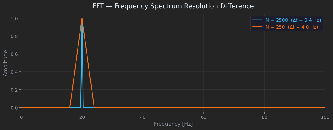
Fewer samples produce a coarser frequency spectrum. The orange trace (10× fewer samples) shows significantly wider peaks.

This matters most in vibration-based condition monitoring, where components separated by only a few hertz must be distinguished. Imagine two vibration sources at 18 Hz and 22 Hz — with insufficient resolution they collapse into a single 20 Hz peak and become indistinguishable:

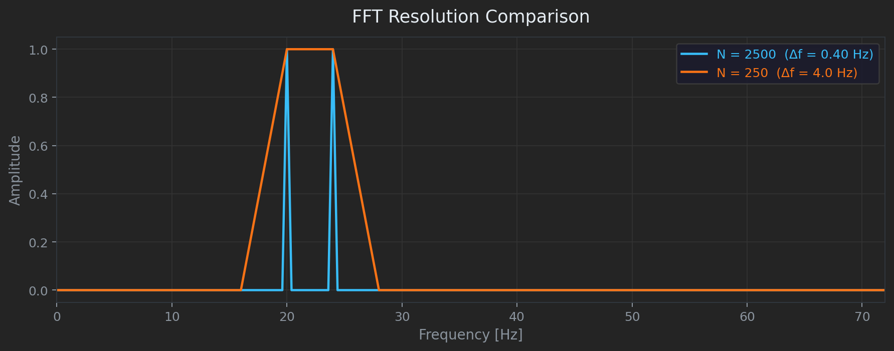
When frequency resolution is too low, the 18 Hz and 22 Hz components merge into a single peak — impossible to differentiate.

These were simulated examples. The three plots below show real data measured with an ADXL345 accelerometer at 800 Hz, using FFT buffer sizes of 128, 1024, and 4096 samples. The measurements were taken separately so they are not identical — but the difference in resolution is clearly visible:

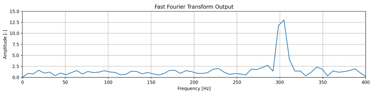
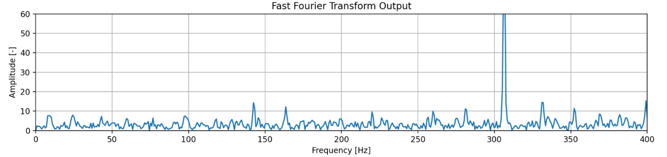
ADXL345 at 800 Hz — FFT buffer sizes of 128, 1024, and 4096 samples. Larger buffers produce sharper, narrower peaks.

More samples means better resolution — but also longer acquisition time and more data to store and process. This tradeoff must be considered carefully in real-time and embedded applications.

Maximum measurable frequency — sampling rate

While the number of samples controls resolution, the sampling frequency determines the highest frequency that can be correctly measured. This is defined by the Shannon-Nyquist theorem:

Nyquist limit:

If the sampling frequency is 1000 Hz, the maximum frequency that can be measured is 500 Hz. In practice the industry guideline is to sample at 5–10× the highest frequency of interest, not just 2×, to provide a safety margin.

When a signal contains frequencies above the Nyquist limit, those components cannot be correctly represented and fold back into the spectrum at lower frequencies. This effect is called aliasing. The example below shows a 90 Hz signal sampled at only 100 Hz — well below the required 180 Hz minimum. The result is a ghost component appearing at 10 Hz, which does not exist in the real signal:

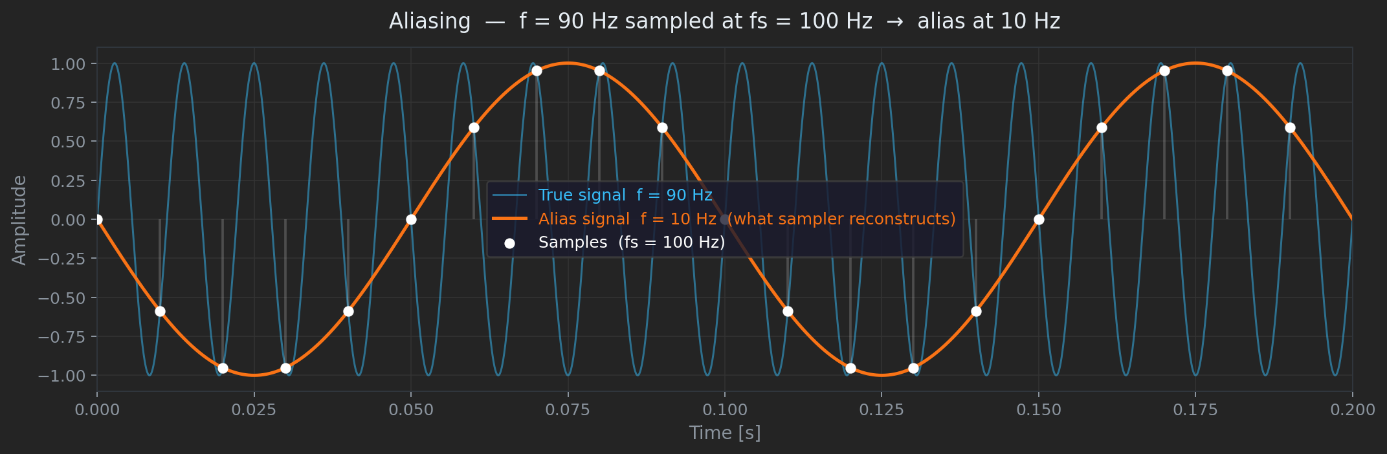
Aliasing: a 90 Hz signal sampled at 100 Hz folds back into the spectrum as a fake 10 Hz component.

To prevent aliasing, the signal is passed through an anti-aliasing filter — a low-pass filter applied before sampling that removes all content above the Nyquist limit.

Real-world example — ADXL345 on a kitchen mixer

I used an ADXL345 accelerometer connected to an STM32 microcontroller to record vibration data from a kitchen mixer. Its rotational speed can be changed manually, which makes it a convenient source of varying vibration frequencies. Python scripts running on a PC plot both the FFT spectrum and a spectrogram in real time — allowing you to see how the frequency content changes over time as the speed varies.

The sampling frequency was set to 800 Hz with an FFT buffer of 128 samples. The small buffer was chosen to achieve good time resolution on the spectrogram — at the cost of lower frequency resolution (df = 800 / 128 = 6.25 Hz per bin).

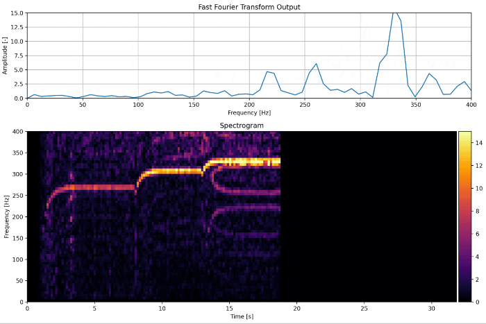
Real-time FFT and spectrogram from an ADXL345 accelerometer on a kitchen mixer. STM32 + Python, 800 Hz sampling, 128-sample FFT buffer.

In the spectrogram the bright horizontal line tracks the dominant vibration frequency as the mixer speed changes. At higher speeds, additional components appear at lower frequencies — these are aliases of high-frequency harmonics that exceeded the 400 Hz Nyquist limit and folded back into the visible range of the spectrum.