Digital Filters Explained

In practice, no measured signal is perfectly clean. Noise, interference, and unwanted frequency components are always present. Digital filters selectively suppress what should not be there — leaving only the signal of interest.

Digital filters — how they work

Filters selectively pass or block parts of a signal based on frequency. Whether the goal is removing electrical noise, isolating a vibration frequency, or cleaning up sensor data, they are one of the most fundamental tools in digital signal processing.

Basic, but important parameters:

• Cutoff frequency (−3 dB point) — the frequency at which the filter begins to attenuate the signal. At this point the signal power is reduced by half.
• Roll-off — defines how sharply the filter suppresses frequencies beyond the cutoff. Higher attenuation means a steeper, narrower transition band and a more precise filter.

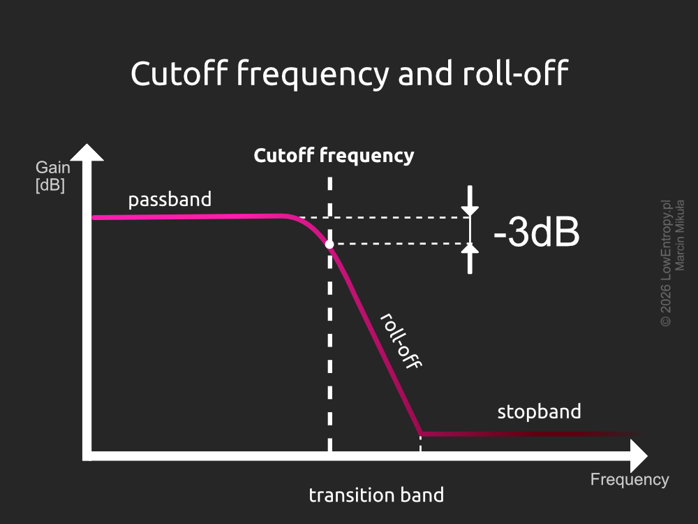
The −3 dB point marks where signal power drops to half its passband value.

Types of filters

There are four main types of filters. A low-pass filter (LPF) allows low-frequency components to pass while attenuating higher frequencies. A high-pass filter (HPF) does the opposite — it passes high frequencies and attenuates the low ones.

A band-pass filter (BPF) allows only a specific range of frequencies to pass, blocking everything outside that range. A band-stop filter (BSF) is the opposite — it attenuates a specific frequency range while passing everything else. When the blocked range is very narrow, a band-stop filter is commonly called a notch filter.

The figure below shows all four filter types applied to the same input signal — built from multiple sine waves of varying amplitude with Gaussian noise added.

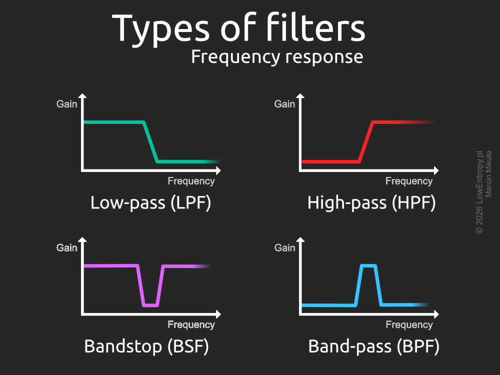
Low-pass, high-pass, band-pass, and band-stop filters applied to a composite noisy signal.

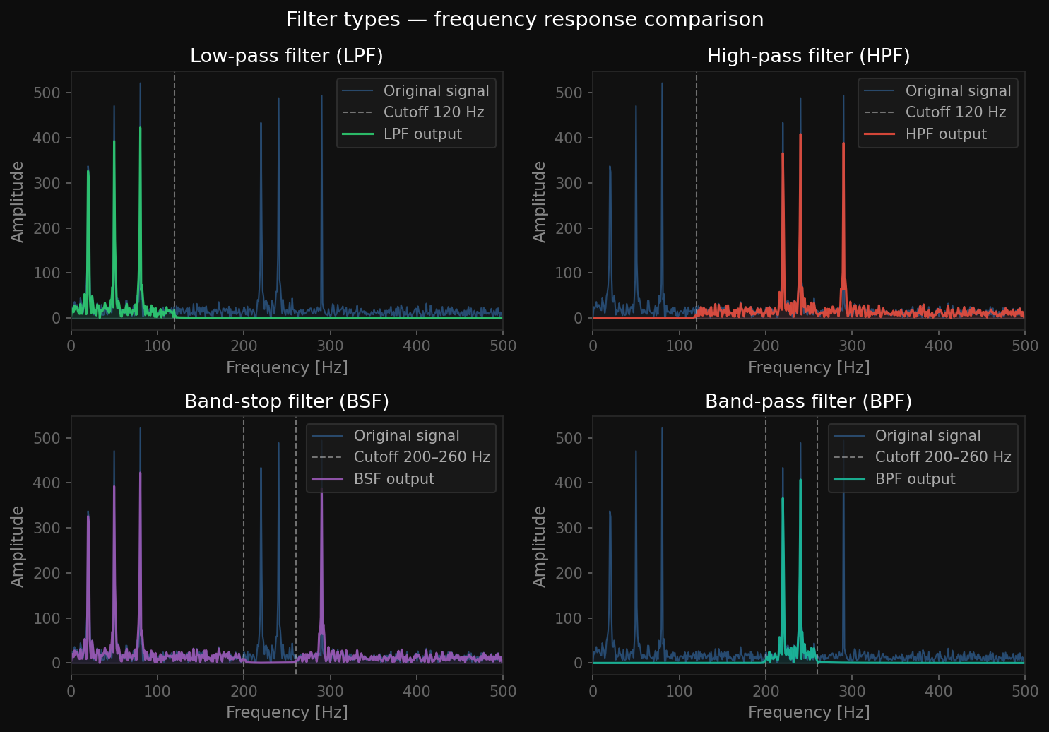
Frequency-domain comparison of all four filter types — LPF, HPF, BPF, and BSF — applied to the same input signal. Each filter passes only its intended frequency range.

How digital filters are designed

FIR filters

FIR (Finite Impulse Response) filters use only current and past inputs to produce a finite response — which is why they are called non-recursive. The input signal x[n] enters the filter, where it is split into delayed copies. Each copy is multiplied by a corresponding filter coefficient. These weighted samples are then summed to produce the filtered output y[n].

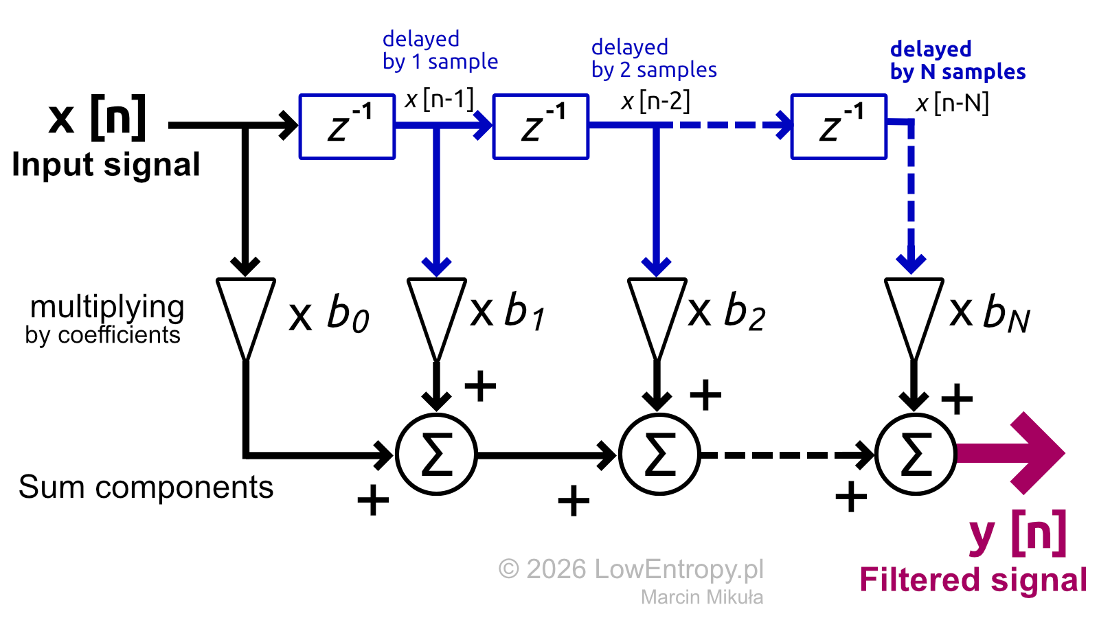
FIR filter structure — delayed input samples multiplied by coefficients and summed.

FIR filter equation:

Advantages

• Always stable and predictable.
• Linear phase response — all frequency components are delayed equally, so the signal is not phase-distorted.

Disadvantages

• Introduce more delay than IIR filters — a longer kernel means more samples must be processed before the output is computed.
• Require more memory and computation — all coefficients must be stored, and each output sample requires as many multiplications as there are taps.

The number of taps (N) defines the length of the filter kernel. A higher tap count produces sharper filtering — at the cost of increased delay and computation.

IIR (Infinite Impulse Response) filters

IIR filters use feedback from past outputs. An IIR filter can be seen as two FIR filters — one in the feedforward path and one in a closed feedback path. They work together as a single unit and cannot be separated.

Starting with the feedforward loop — it works similarly to FIR filters: delayed input samples are multiplied by coefficients and summed.

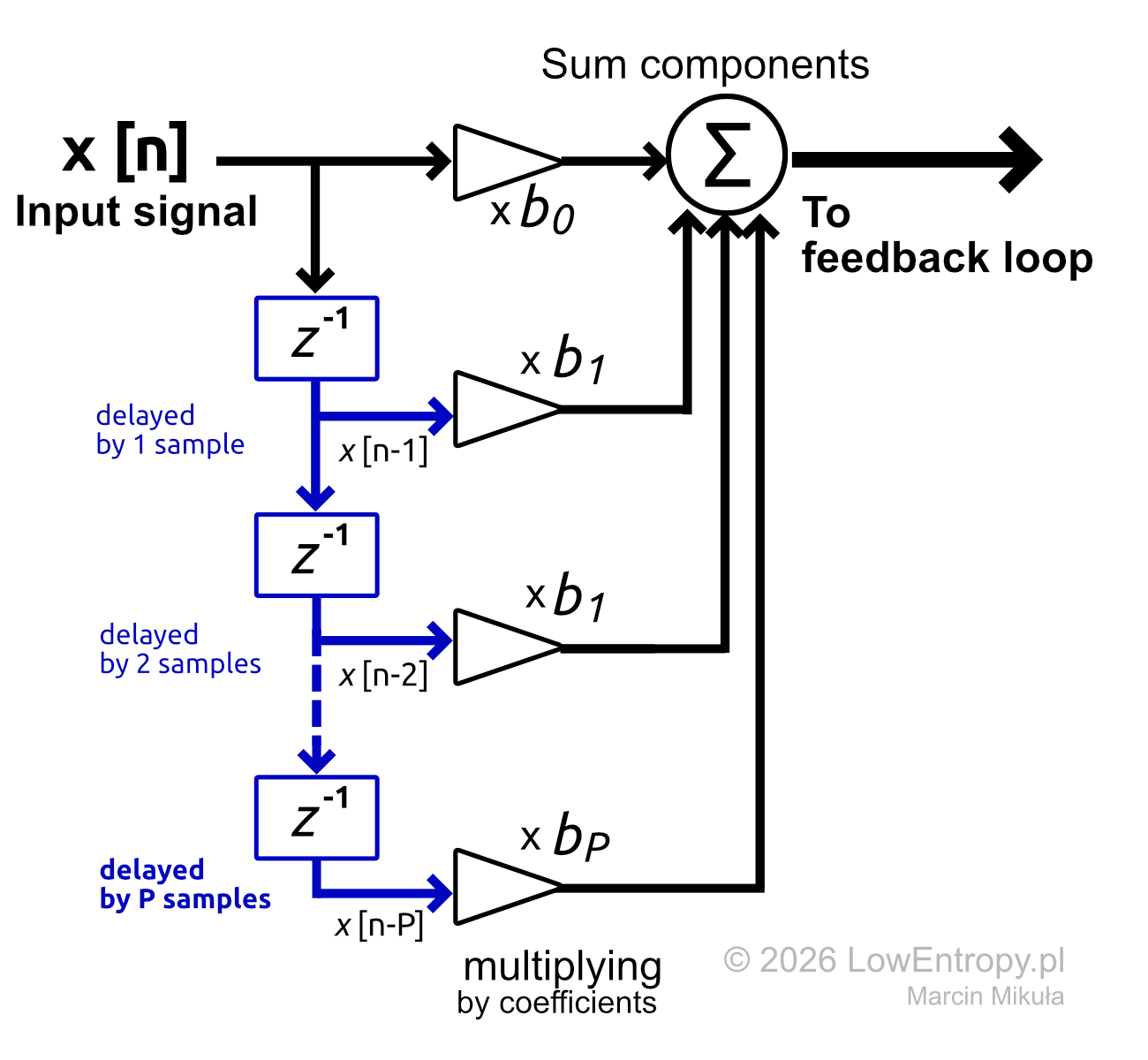
IIR feedforward path — structurally identical to an FIR filter.

The feedback path operates on past output samples — structurally similar to the feedforward path, but entering the summation node with a negative sign. Equivalently, the feedback coefficients a₁, a₂, ..., a_Q can be treated as negative values.

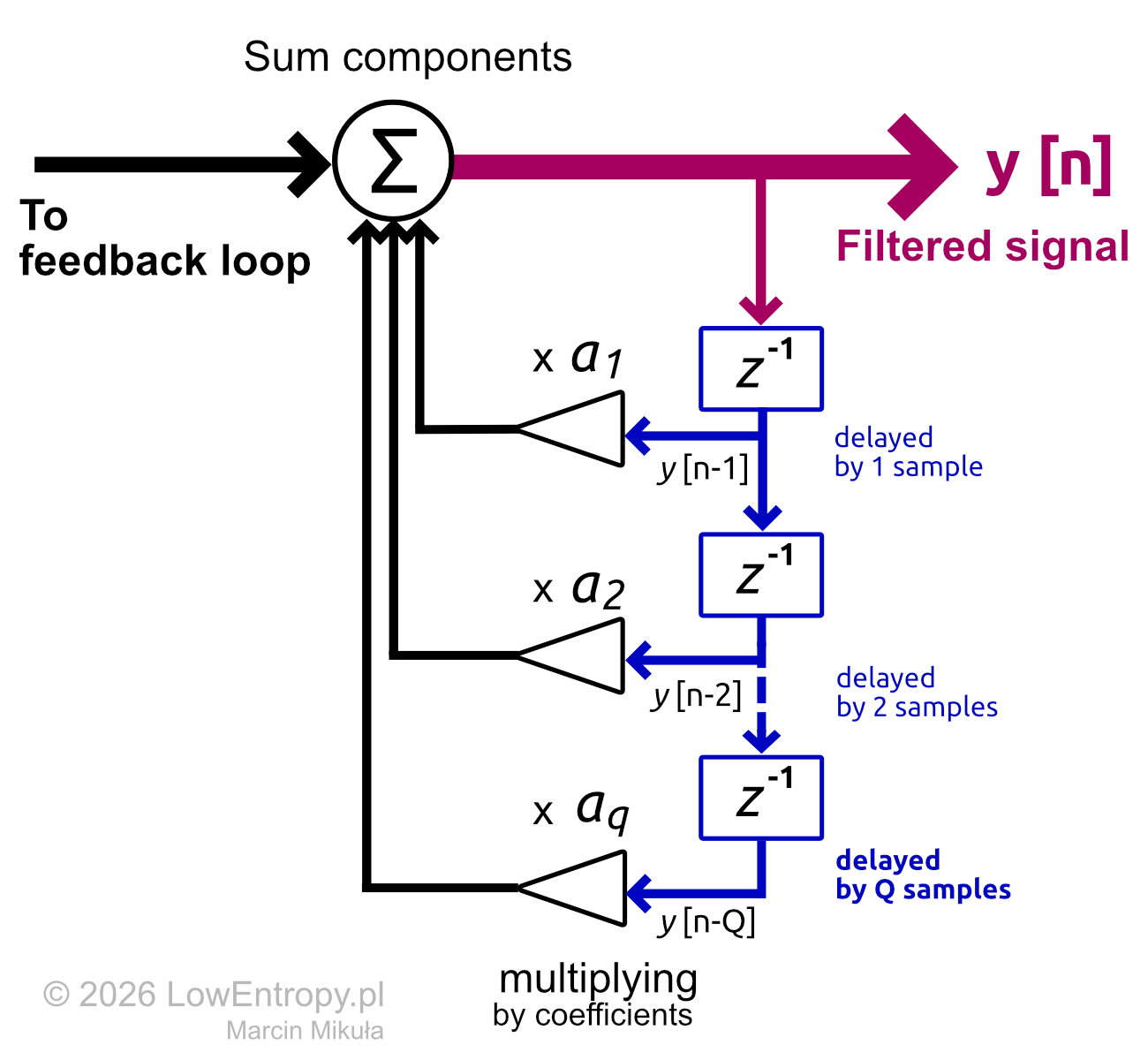
IIR feedback path — past output samples fed back into the summation node.

As shown below, both paths share a single summation node.

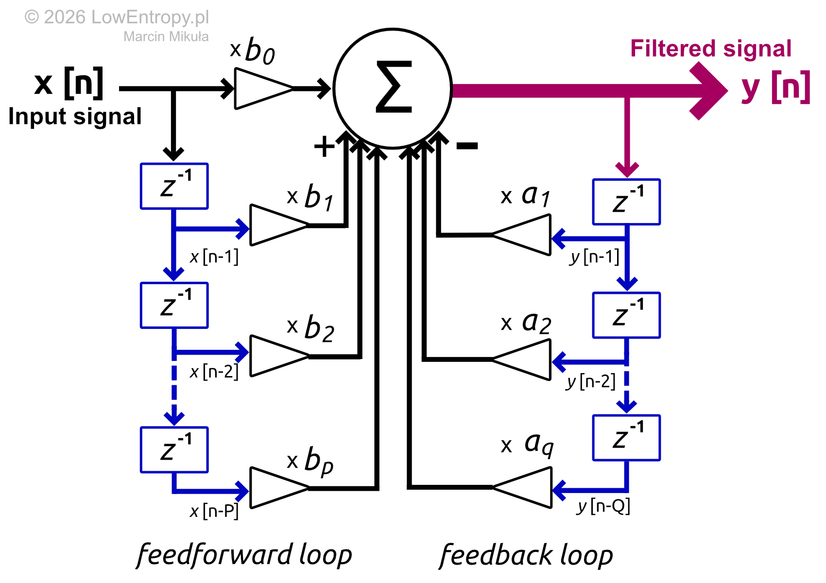
Complete IIR filter structure — feedforward and feedback paths meeting at a single node.

IIR filter equation:

The main advantage of IIR filters is efficiency — for the same filtering performance, an IIR design typically requires far fewer coefficients than an equivalent FIR filter, meaning less memory and fewer arithmetic operations per sample. However, IIR filters are sensitive to numerical errors and coefficient rounding, which can cause instability. Stability must always be verified — a common method is to plot the filter's poles on the Z-plane. If all poles lie strictly inside the unit circle, the filter is stable. Pole-zero analysis and the Z-plane will be covered in a separate article.

Common IIR filter designs

There are several well-established IIR filter designs, each with different characteristics in the passband and stopband:

• Butterworth — maximally flat passband with no ripple. The most common general-purpose choice.
• Chebyshev Type I — steeper rolloff than Butterworth for the same order, but with ripple in the passband.
• Chebyshev Type II — flat passband with ripple in the stopband. A good compromise when passband smoothness matters.
• Elliptic — the steepest rolloff of all, but with ripple in both bands. Used when the transition band must be as narrow as possible.

A detailed comparison of these filter designs will be covered in a separate article.

Advantages

• Much lower order than equivalent FIR filters — fewer coefficients, less memory, faster computation.
• Near-instant response — no startup delay caused by a long kernel.
• Well-established analog prototype designs can be converted directly to digital form.

Disadvantages

• Non-linear phase response — different frequency components are delayed by different amounts, which can cause phase distortion.
• Sensitive to numerical errors — coefficient rounding can cause instability, especially in fixed-point implementations.
• Stability must always be verified.

How an FIR filter works — step by step

The animation below illustrates how an FIR filter works on a simulated signal. The kernel slides along the time axis and for each step the output is computed. Two FIR kernels of different lengths are shown — to compare how quickly they settle and how well they perform.

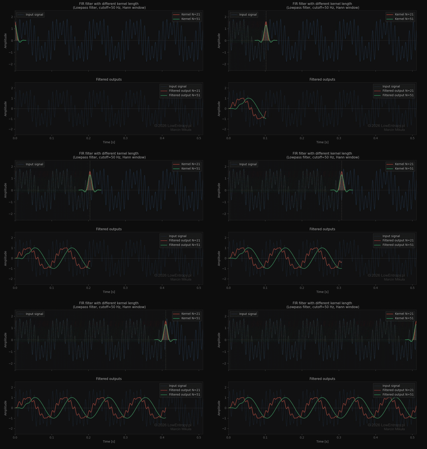
Two FIR filters with different kernel lengths applied to the same signal in real time.

The green filter (larger number of taps, longer kernel) has a greater delay compared to the red one — more samples must be processed before the filter produces the desired output. On the other hand, the red filter (N = 21, smaller kernel) performs worse and does not attenuate high-frequency components as effectively.

This illustrates the core tradeoff in FIR filter design — speed versus quality.

The FFT below shows the same signal in the frequency domain. Note that the signal filtered by the red kernel (N = 21) still has some high-frequency content remaining in its spectrum — which corresponds to what we see in the time domain above.

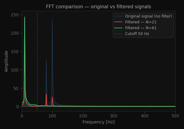
FFT of the original signal and both filtered outputs — the shorter kernel (N = 21) leaves more residual high-frequency energy.

FIR & IIR filter — comparison in Python

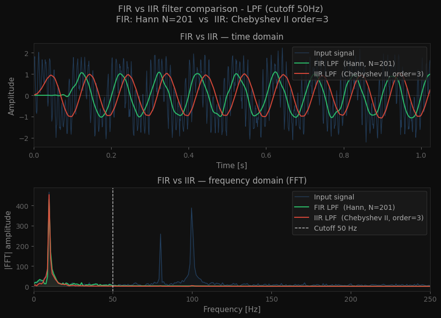
FIR (green, N=201) vs IIR (red, Chebyshev II, order=3) — time domain and frequency domain, low-pass at 50 Hz.

The plot above shows both filters applied to the same input signal — a low-pass filter with a cutoff frequency of 50 Hz. In the time domain, the difference is immediately visible. The FIR filter (green, N=201) introduces a noticeable startup delay — the output takes some time to settle because the kernel must accumulate enough samples before producing a valid result. The IIR filter (red, Chebyshev II, order=3) responds almost instantly, with no visible startup delay.

In the frequency domain, both filters effectively suppress frequencies above 50 Hz — the 80 Hz and 100 Hz components are clearly attenuated in both outputs. However, the IIR filter achieves this with only 3 coefficients, while the FIR filter requires 201. This illustrates the core tradeoff — FIR filters are stable and predictable with linear phase, but require significantly more coefficients. IIR filters are compact and fast, but introduce phase distortion and require stability verification.

Real-world example — ADXL345 accelerometer data

I implemented FIR filters on an STM32 microcontroller devboard using CMSIS libraries, paired with an ADXL345 accelerometer mounted on a kitchen mixer as a source of vibrations. A band-pass filter with a passband of 320–340 Hz was implemented. The filter is toggled by a physical button on the STM32 board — pressing it switches filtering on and off in real time.

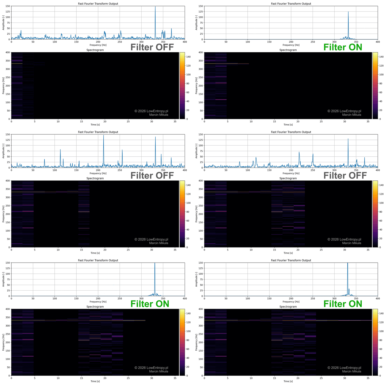
Band-pass FIR filter toggled on/off in real time — STM32 + ADXL345 on a kitchen mixer.

It is clear that the peak frequency remains visible while all other frequencies are attenuated as if they were not present. On the spectrogram, a single horizontal line is visible — only the 320–340 Hz band passes through.