Spectral Leakage & Windowing

When you apply FFT to a real signal, you rarely get clean, sharp peaks. Instead, the energy of a single frequency component often spreads across neighboring bins, polluting the spectrum. This phenomenon is called spectral leakage — and understanding why it happens is the first step to controlling it.

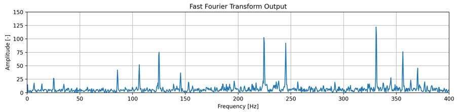
Example of spectral leakage — a single frequency component spreads across multiple FFT bins instead of appearing as a single sharp peak.

Why does spectral leakage appear?

FFT assumes that the captured signal repeats perfectly and infinitely — but in practice we only capture a finite slice. When that slice doesn't end cleanly, a discontinuity is introduced at the edges. There are two main scenarios that cause leakage:

• The signal frequency falls between FFT bins. If the FFT resolution is 1 Hz and the signal is at 22.5 Hz, there is no bin at exactly 22.5 Hz — the energy leaks into adjacent bins.
• The captured window doesn't contain an integer number of cycles. If you capture 2.5 cycles of a signal, the start and end of the window don't match — creating an artificial edge discontinuity.

Scenario 1 — frequency between bins

Consider two signals: one at 20.0 Hz and one at 22.5 Hz, both sampled at F_s = 1000 Hz with N = 1000 samples. The FFT resolution is df = F_s / N = 1 Hz, so the frequency bins are at 0, 1, 2 ... 20, 21, 22, 23 Hz — but there is no bin at 22.5 Hz.

In the time domain, the 22.5 Hz signal also does not complete an integer number of cycles within the capture window — the end of the window does not match the start:

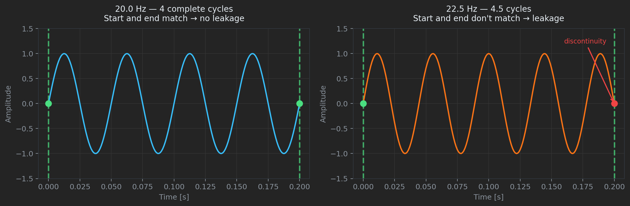
The 20 Hz signal fits neatly into the window; the 22.5 Hz signal does not — creating an edge discontinuity.

In the frequency domain this mismatch is clearly visible. The 20 Hz component produces a clean sharp peak, while the 22.5 Hz component spreads its energy across the surrounding bins:

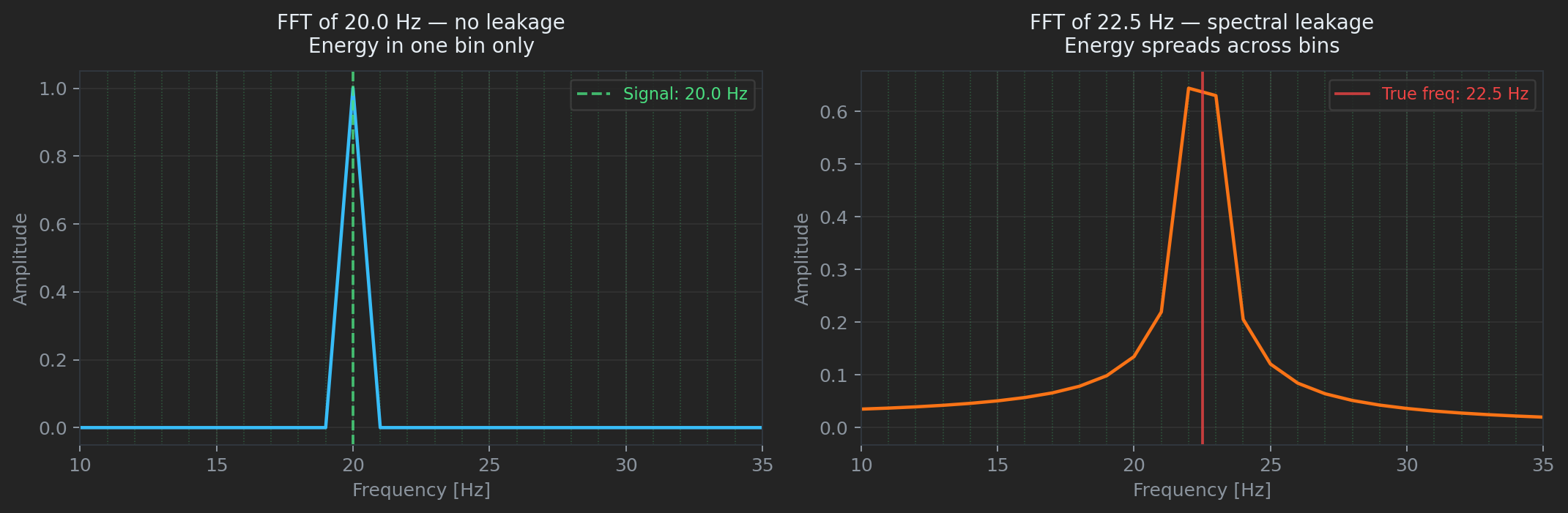
The 20 Hz component lands exactly on a bin — clean peak. The 22.5 Hz component falls between bins and leaks into its neighbors.

Scenario 2 — non-integer number of cycles

Even if the signal frequency is perfectly aligned with the FFT bins, leakage can still occur if the captured window doesn't contain a whole number of cycles. The signal appears to jump at the boundary — and FFT treats that jump as broadband energy:

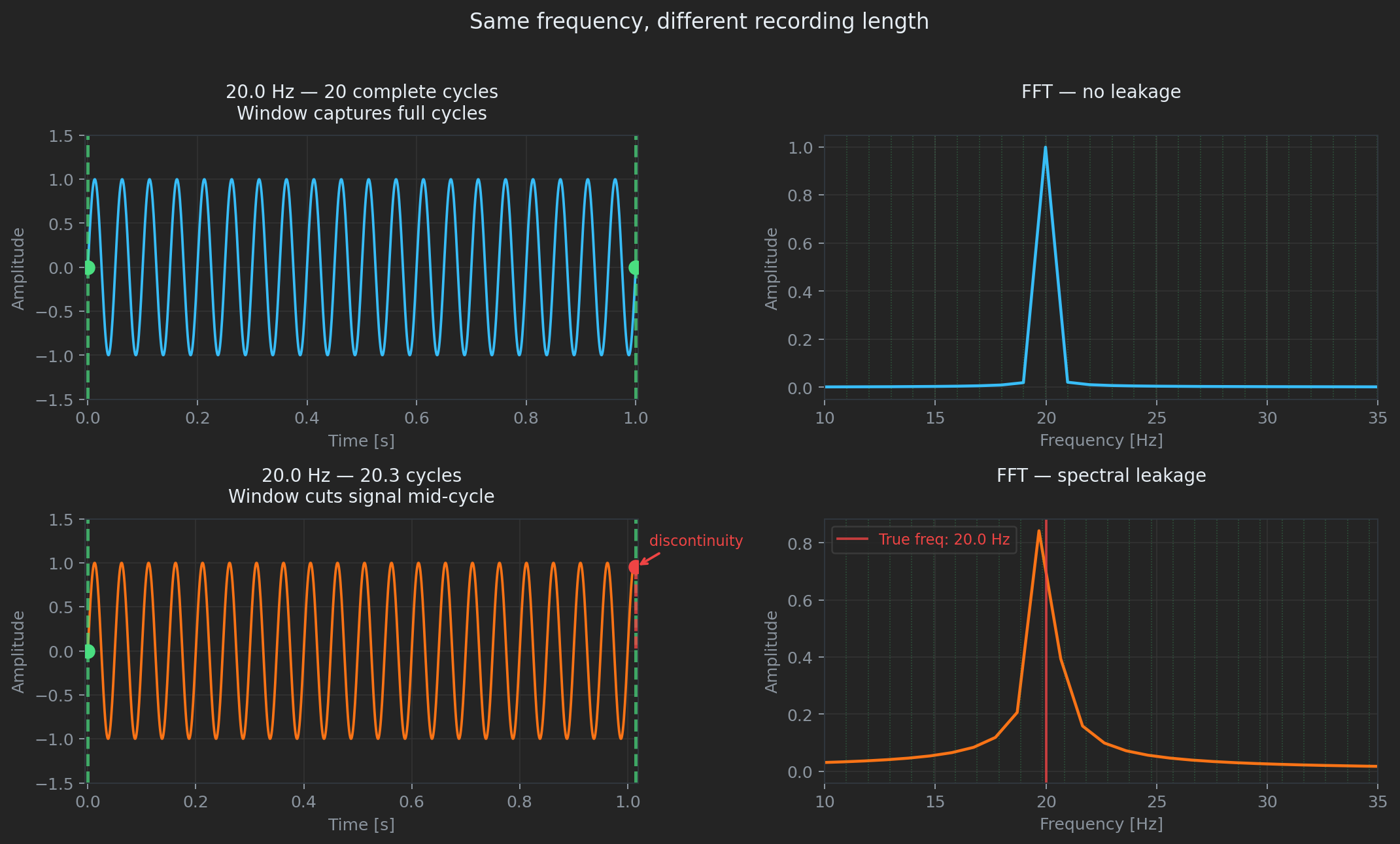
A non-integer number of cycles in the capture window creates a discontinuity at the edges — leading to leakage in the FFT output.

Windowing — how it helps

A window function is a weighting applied to the signal before FFT. It gradually tapers the amplitude to zero at both edges of the capture window, eliminating the sharp discontinuity that causes leakage. The most commonly used window is the Hann window.

The comparison below shows the same signal processed without a window and with a Hann window applied. The leakage — the wide skirt of energy around the peak — is dramatically reduced:

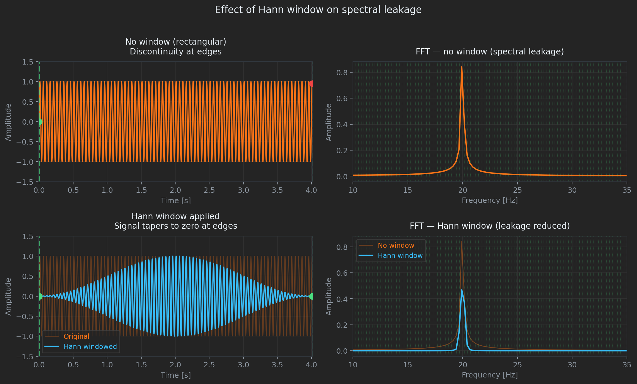
Left: raw FFT without windowing — heavy spectral leakage. Right: FFT with Hann window applied — leakage largely eliminated.

In practice, FFT is often applied to a continuous stream of data in overlapping slices. The Hann window is commonly used in 90% of cases — it is applied independently to each frame before the FFT is computed. Let's simulate that scenario and see the results.

Types of window functions

Different window functions offer different trade-offs between frequency resolution and leakage suppression. The plot below shows the shapes of three common windows:

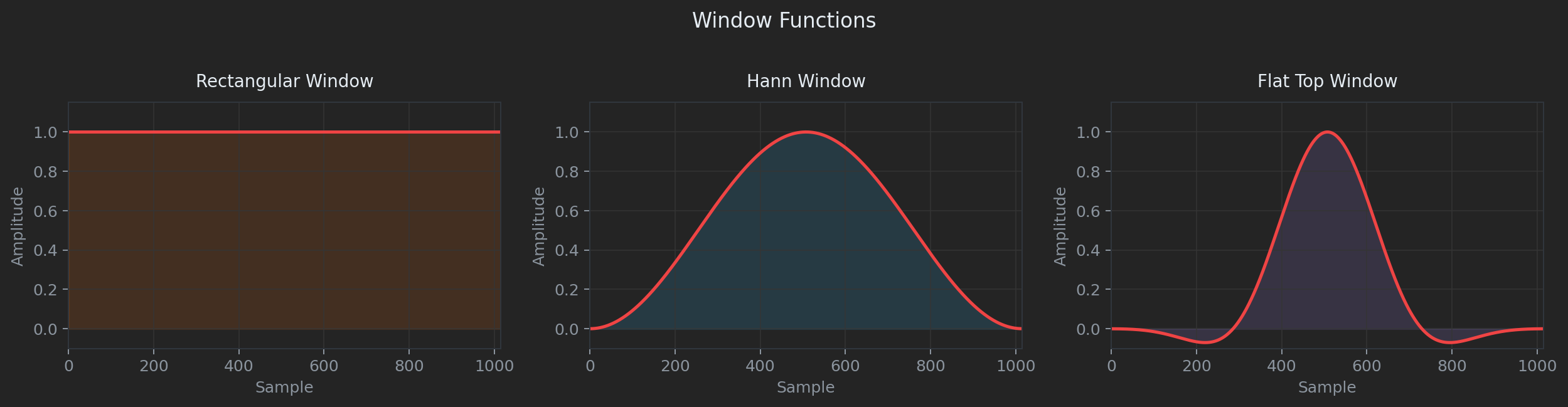
Shapes of three common window functions — rectangular, Hann, and flat top.

Rectangular window

The rectangular window is effectively no windowing at all — every sample in the frame is weighted equally at 1.0. It gives the best frequency resolution but provides no protection against spectral leakage. Useful only when the signal is guaranteed to contain an integer number of cycles in the window.

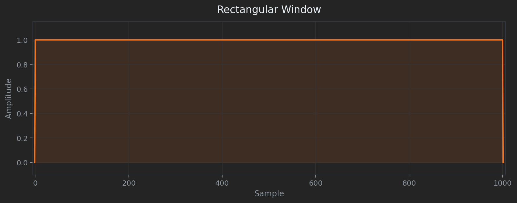
Rectangular window — flat weighting, no edge tapering, highest leakage.

Hann window

The Hann window (sometimes called Hanning) is the go-to choice for the vast majority of FFT applications. It smoothly tapers to zero at both edges using a raised cosine shape, effectively eliminating edge discontinuities.

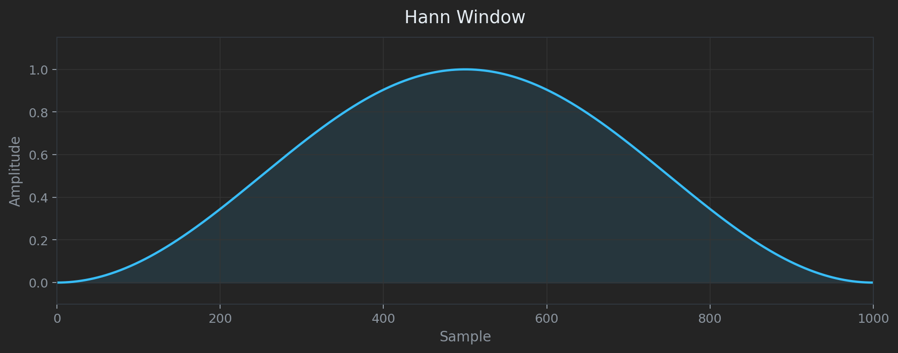
Hann window — smooth cosine taper, good balance between resolution and leakage suppression.

Hann window equation:

Flat top window

The flat top window is designed for accurate amplitude measurement. Its passband is nearly flat, meaning signal amplitude is preserved faithfully — at the cost of much wider peaks and lower frequency resolution. It is the preferred choice when you need to measure the exact amplitude of a component rather than resolve nearby frequencies.

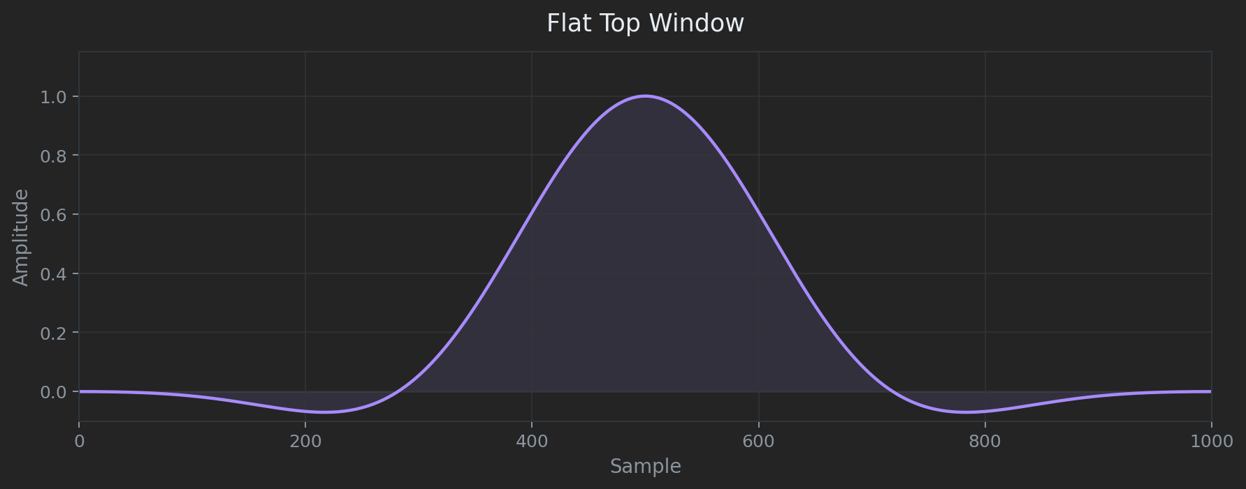
Flat top window — wide, flat passband preserves amplitude accuracy at the cost of frequency resolution.

Flat top window equation:

How the windowed signal looks

When a window is applied repeatedly to overlapping slices of a continuous signal, each slice is shaped before going into the FFT. The visualization below shows successive windowed frames — note how each frame tapers smoothly to zero at both ends regardless of what the underlying signal is doing:

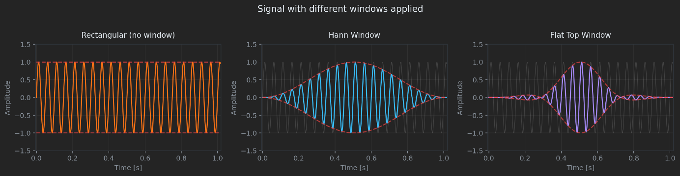
Overlapping windowed slices of a signal. Each frame is independently tapered before FFT is applied.

The tradeoff with windowing

Applying a window is not free. Any window other than rectangular attenuates the signal — samples near the edges are multiplied by values close to zero, which reduces the total energy entering the FFT. This means the amplitude of peaks in the spectrum will be lower than the true amplitude.

To compensate, a correction factor is applied after the FFT, normalizing the output based on the known energy loss of the chosen window. Most signal processing libraries handle this automatically.

The key trade-offs to keep in mind:

• Rectangular — best frequency resolution, worst leakage. Only suitable when signal fits perfectly in the window.
• Hann — good leakage suppression, slight resolution loss. Best general-purpose choice.
• Flat top — best amplitude accuracy, lowest frequency resolution. Use when measuring amplitudes, not resolving frequencies.

Real-world example — ADXL345 accelerometer

I used an ADXL345 accelerometer connected to an STM32 microcontroller to capture vibration data from a kitchen mixer. A Python script computes FFT and renders both a spectrum and a spectrogram in real time. A physical button on the STM32 board toggles the window function on and off — making it possible to see the effect of windowing instantly on live data.

First, without any window function applied. The dominant frequency peak is clearly visible but has wide skirts — spectral leakage spreading energy into neighboring bins:

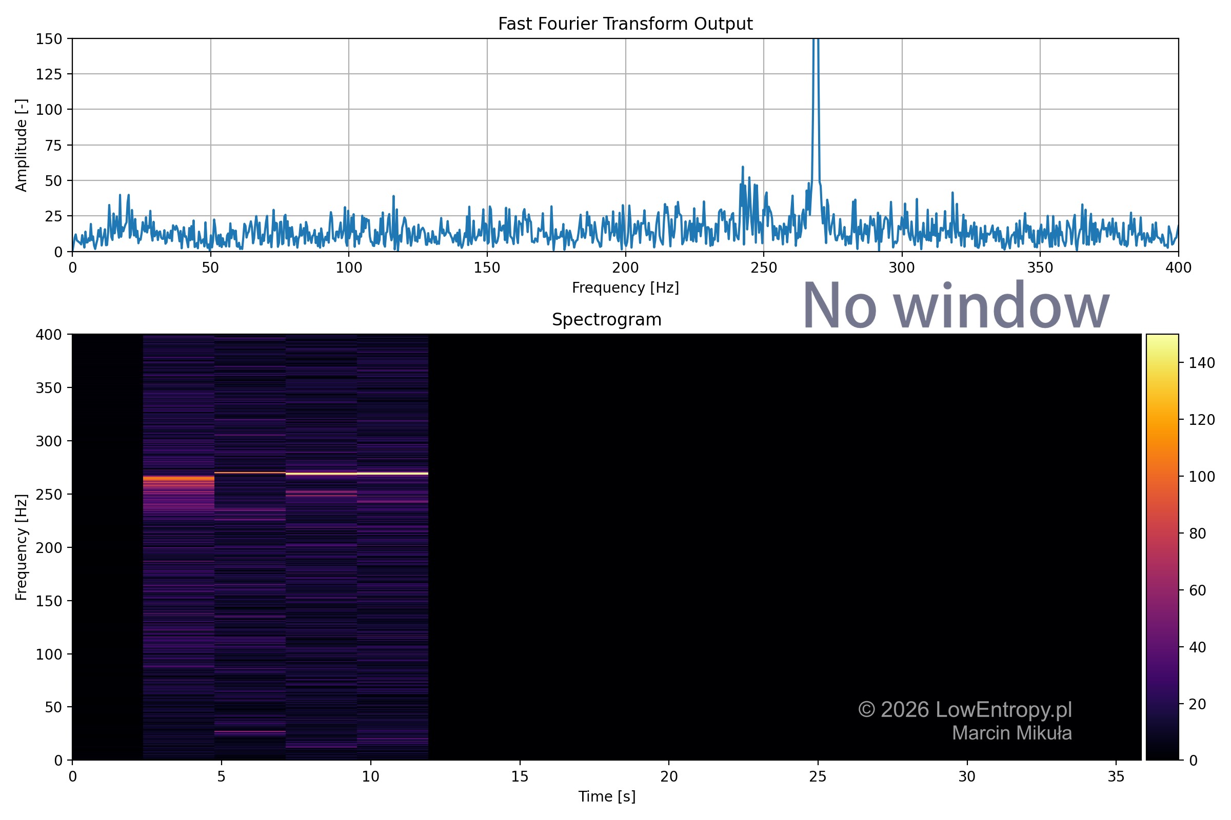
No window applied — the dominant peak has wide leakage tails spreading into neighboring frequency bins.

After pressing the button to enable the Hann window, the leakage drops immediately. The peak becomes narrower and the spectrum around it is significantly cleaner:

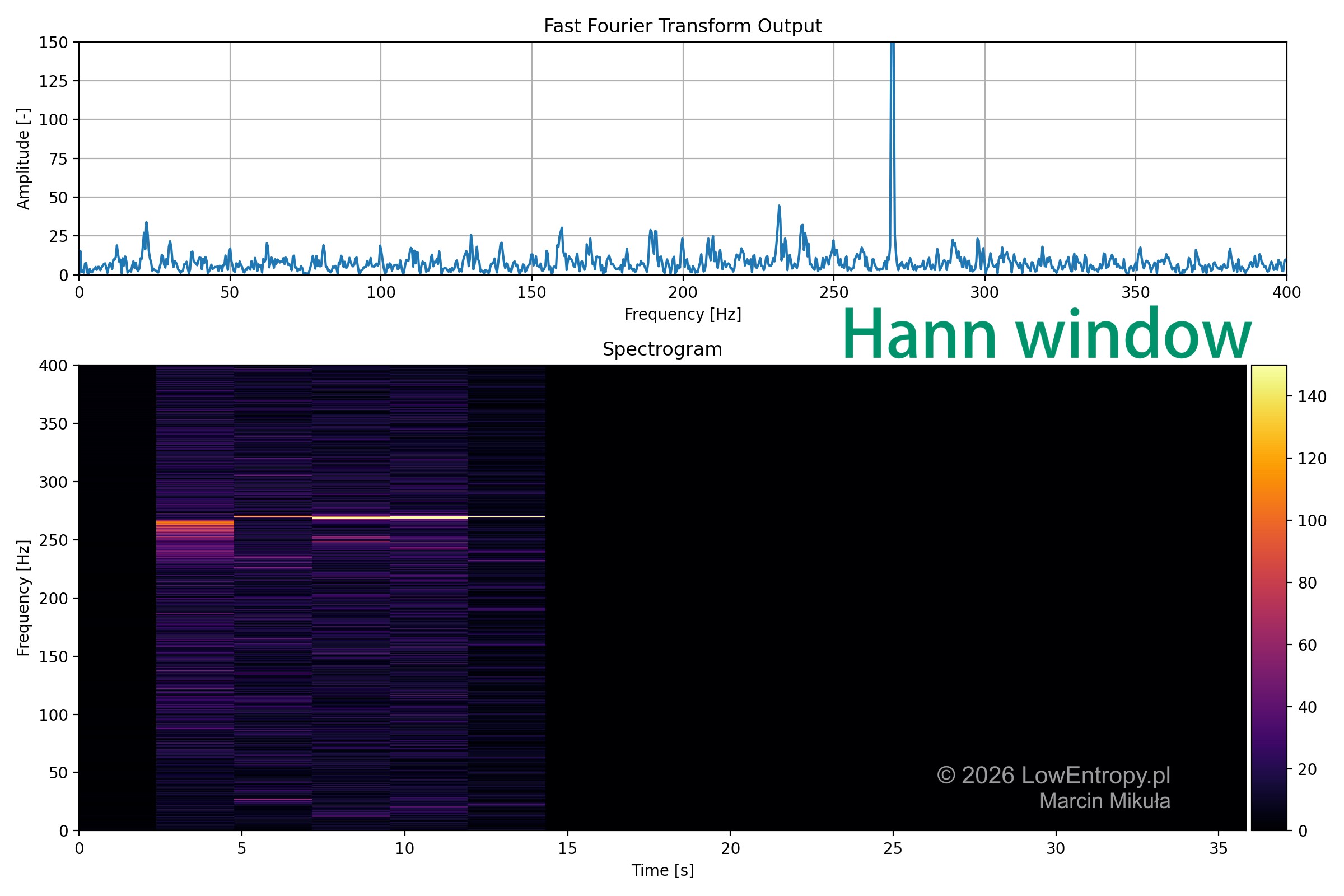
Hann window applied — leakage suppressed, the peak is sharper and the noise floor around it drops noticeably.

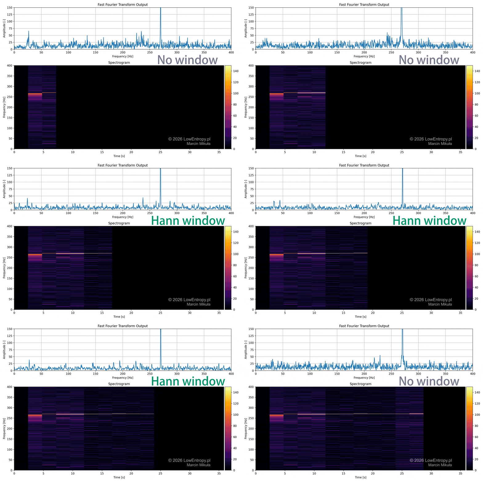
Real-time spectrogram showing the moment the Hann window is toggled on — the leakage drops instantly and the frequency band becomes sharper and cleaner.