
Contents
What is a PID controller?
A PID controller is a control loop mechanism used to manage processes and machines that require automatic adjustment. It allows a physical device to follow a given setpoint: for an electric motor this could be a target rotational speed, for the carriage of a 3D printer a specific position along an axis, and for a heater a target temperature.
When a disturbance occurs, the controller adjusts its output signal to bring the measured value back to the setpoint. Such a disturbance might be a motor coming under load, or a drop in ambient temperature.
It is one of the simplest and most widely used types of controllers. It remains the preferred solution in much of industrial automation.
In this article we’ll look at how a PID controller works, and run a few experiments to see how it behaves on a real, physical system.
PID controller - how is it built?
A PID controller can be easily visualised as a block diagram, as shown below:
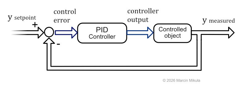
PID controller block diagram - proportional, integral, and derivative paths combined.
The controller consists of three components:
- Proportional part
- Integral part
- Derivative part
Equation of an ideal PID controller and its parameters
e(t) - control error (setpoint − measured value)
Kp - proportional gain
Ti - integral time constant [s]
Td - derivative time constant [s]
But this is just the theory. Because the PID algorithm in modern devices is implemented on digital hardware, it has to be transformed into its discrete form.
PID controller in discrete form
After a few substitutions, the integral becomes the sum of the error, while the differential becomes the difference between the previous and current error values.
∑e[i] - sum (integral) of error
e[k] − e[k−1] - error difference (derivative)
How the parameters affect the PID system response
The main goal was to show how the theory looks in practice. The photograph shows the laboratory setup: a DC motor (Dunkermotor GR63×55) and the power supply. Speed was measured from incremental encoder readings (500 PPR), and the sampling time was set to 50 ms, which is sufficient for this system.
The PID algorithm and data acquisition were implemented on an STM32 microcontroller, while the actuator (a motor driver PCB) was a Cytron MD13S, controlled by the STM32’s PWM output. The controlled variable was rotational speed, in revolutions per minute (RPM).
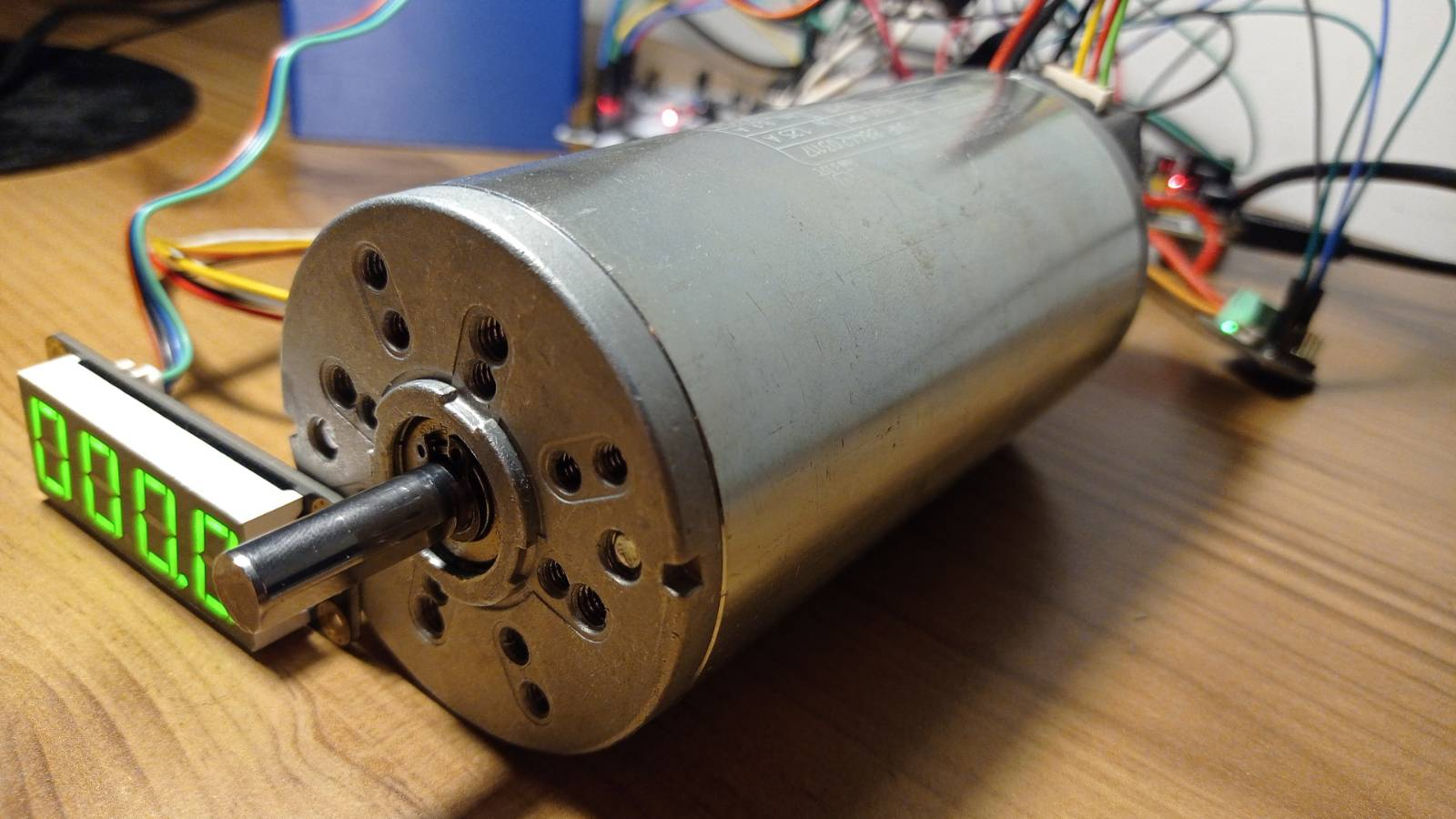
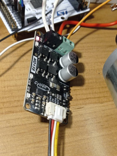
Left: the motor under test (Dunkermotor GR63×55), with measured speed on the green RPM display. Right: the Cytron MD13S motor driver, controlled by the STM32’s PWM output.
Kp - proportional gain
The larger the gain, the more sensitive the controller. As shown in the equation above, it scales all the other components (the integral and derivative parts). The proportional term is proportional to the control error - the difference between the setpoint and measured values. So at the beginning, when a step change in setpoint is applied, the output signal rises immediately.
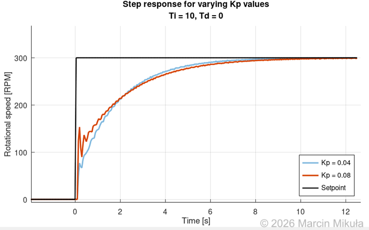
Step response for different proportional gain (Kp) values.
In a P controller without an integral part, it helps reduce the steady-state error, and it does so in a PID controller too. But it has a major disadvantage: it cannot be too large, or the system begins to oscillate and can eventually lose its stability.
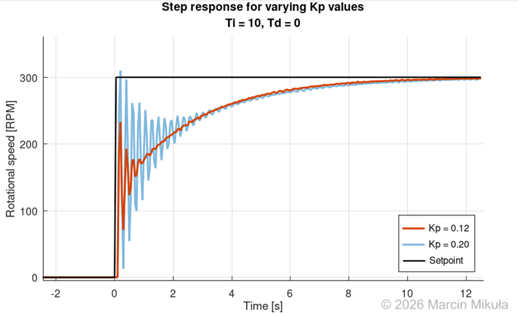
Increasing Kp beyond a certain threshold causes the system to oscillate and lose stability.
Ti - integral time constant
This is a crucial parameter, as it reduces the steady-state error to zero over time. The larger Ti is, the more slowly the integral part acts. Conversely, the smaller Ti is, the more intensively the integral part works. Decreasing this parameter can lead to faster stabilisation of the measured output, but it also affects the stability of the system: if the integral time is too short, the PID response becomes too sensitive and oscillations can appear. As with the proportional gain Kp, this can drive the system into instability.
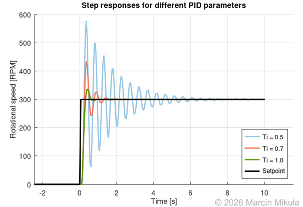
Step response for decreasing Ti values - too short an integral time causes the system to oscillate and eventually lose stability.
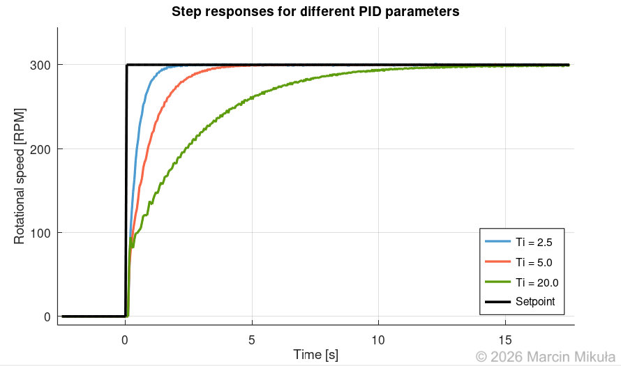
The opposite case: a very large Ti means the system requires much more time to stabilise.
Td - derivative time constant
The derivative part responds to the rate of change of the measured variable and has a positive impact on system stability. Textbooks often present the derivative action as purely beneficial (“improves stability, reduces overshoot”), but the practical reality is that D amplifies high-frequency measurement noise, and is therefore often disabled or heavily filtered in real systems.
Implementation on STM32 microcontroller
The PID output is calculated, and then that output - expressed as a PWM duty cycle - is set. That’s why the code is split into two separate libraries: a PWM output library and a PID library.
Fragment of implementation in embedded C:
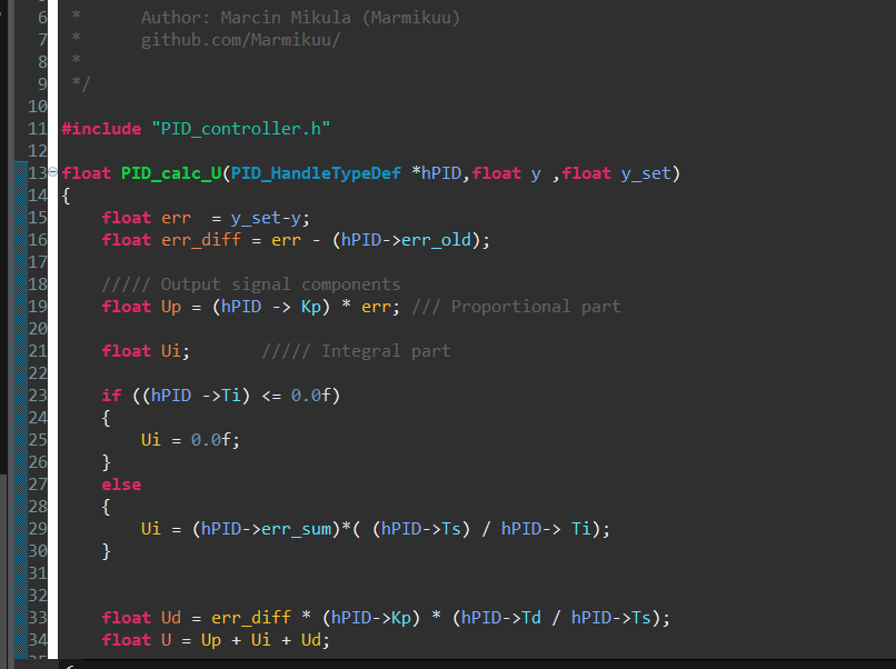
First part: calculating the PID output.
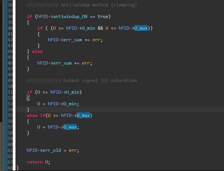
Second part: anti-windup method and output signal saturation.
Unlike in simulations, the controller output must be saturated in a real physical system. The control signal drives an actuator - here, a PWM-controlled motor driver - which in turn drives the plant (the motor). That actuator has hard physical limits: the PWM duty cycle cannot exceed 100% or go below 0%, so the controller output has to be clamped to the range the hardware can actually deliver.
The PID controller and PWM output functions are available in the GitHub repository: github.com/Marmikuu/STM32_Embedded_Control_Systems.
Output signal as a PWM duty cycle
The controller output is expressed as a PWM duty cycle. The following captures show the code responsible for setting the signal, the timer configuration, and the resulting waveform at the microcontroller’s output pin.
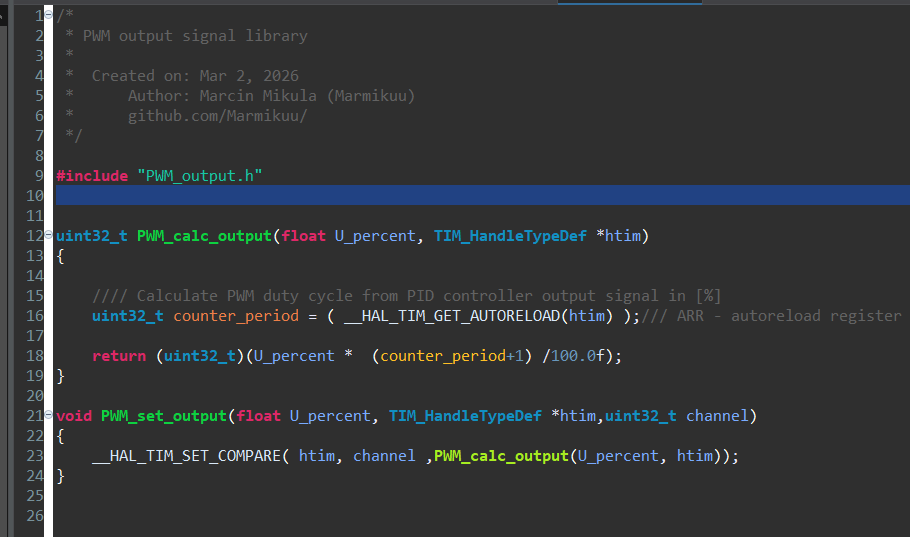
Code fragment responsible for setting the PWM signal’s duty cycle.
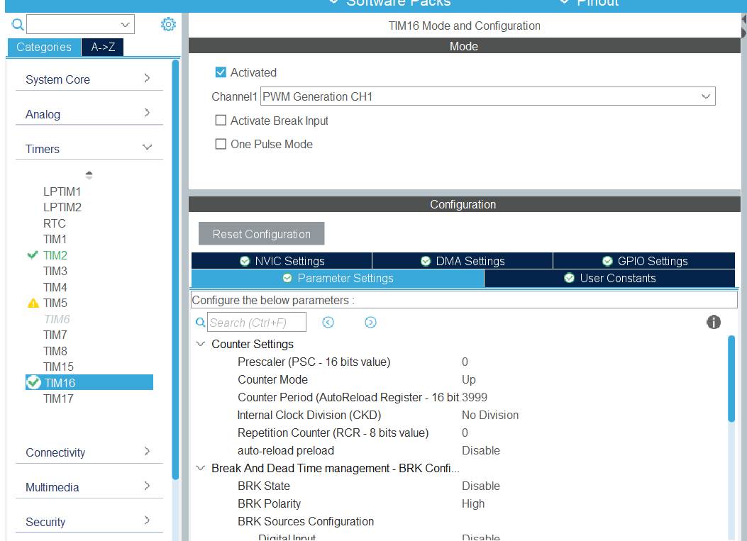
PWM timer configuration in STM32CubeIDE - TIM16 configured to operate at 20 kHz.
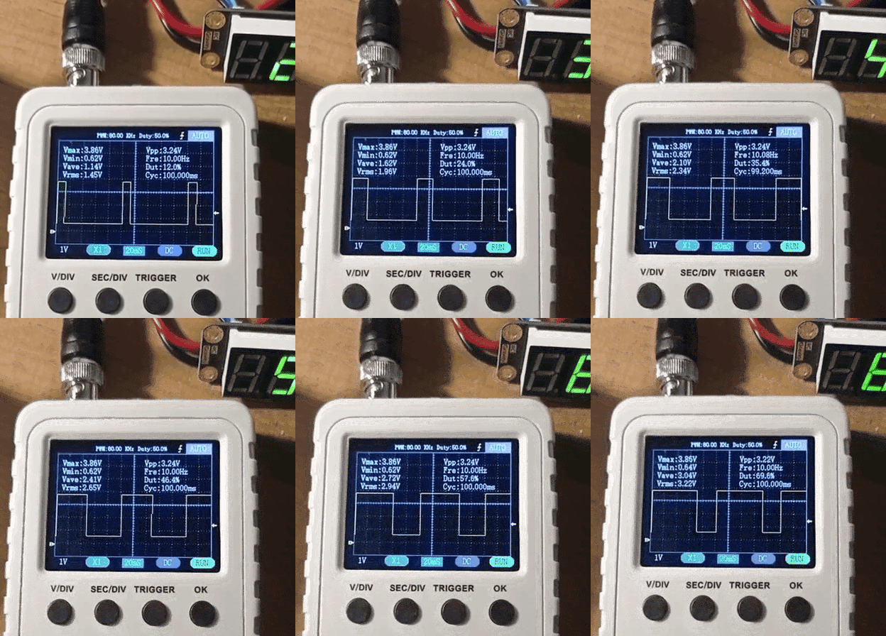
PWM duty cycle gradually changing - captured on oscilloscope.
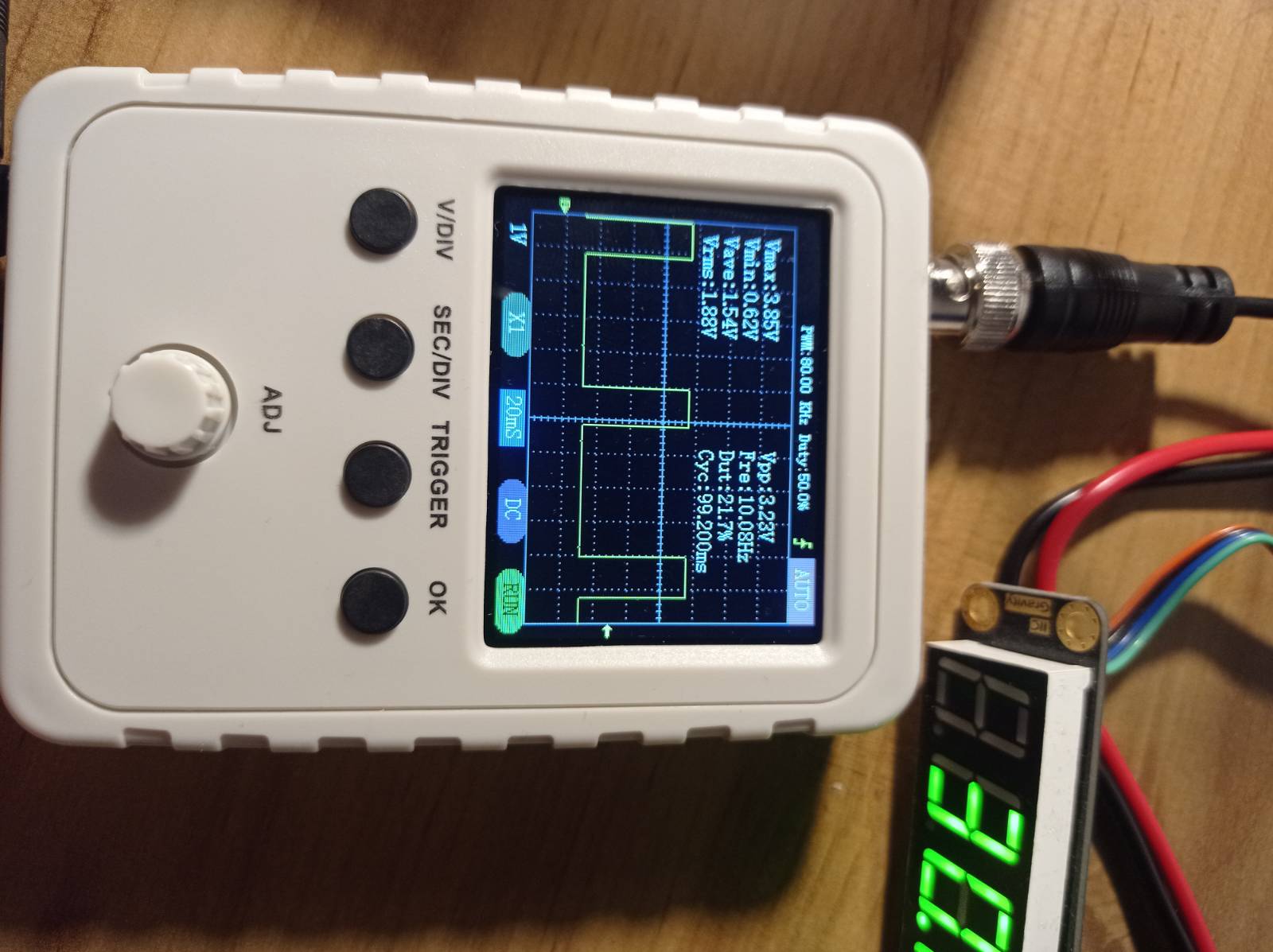
Microcontroller’s PWM signal measured with oscilloscope.
Windup effect and anti-windup methods
The windup effect occurs when the controller’s output signal becomes saturated. This can happen with any real system, since physical actuators always have limits. While the output is saturated, the integral of the control error continues to “wind up” - it keeps accumulating even though the actuator cannot respond. The result is large overshoot and oscillation, and a significantly longer settling time, as shown in the figure below.
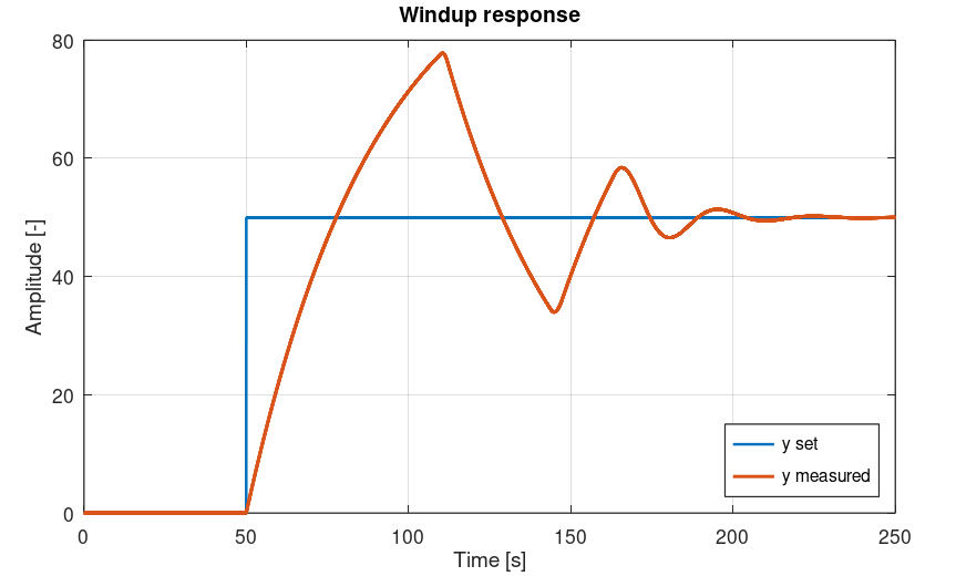
Simulated step response with windup effect - simulation in Octave.
That’s why an anti-windup mechanism is a useful addition. It was described by Karl Åström many years ago and a full description is available in the references section.
There are three well-described anti-windup methods:
- Clamping
- Back calculation
- Limited integration range
In this article only clamping will be described - not only because the idea is straightforward and reliable, but also because it does not depend on any parameter (threshold, coefficients) and therefore needs no tuning.
“Clamping” - the basic anti-windup method
The idea is simple: if the output signal hits saturation boundaries, then error integration should be stopped. This prevents the error sum from becoming large and makes the controller robust to saturation.
Below it is visualised on an animated GIF; the PID with anti-windup applied has much smaller overshoot, and the settling time is much shorter compared to a basic PID without it.
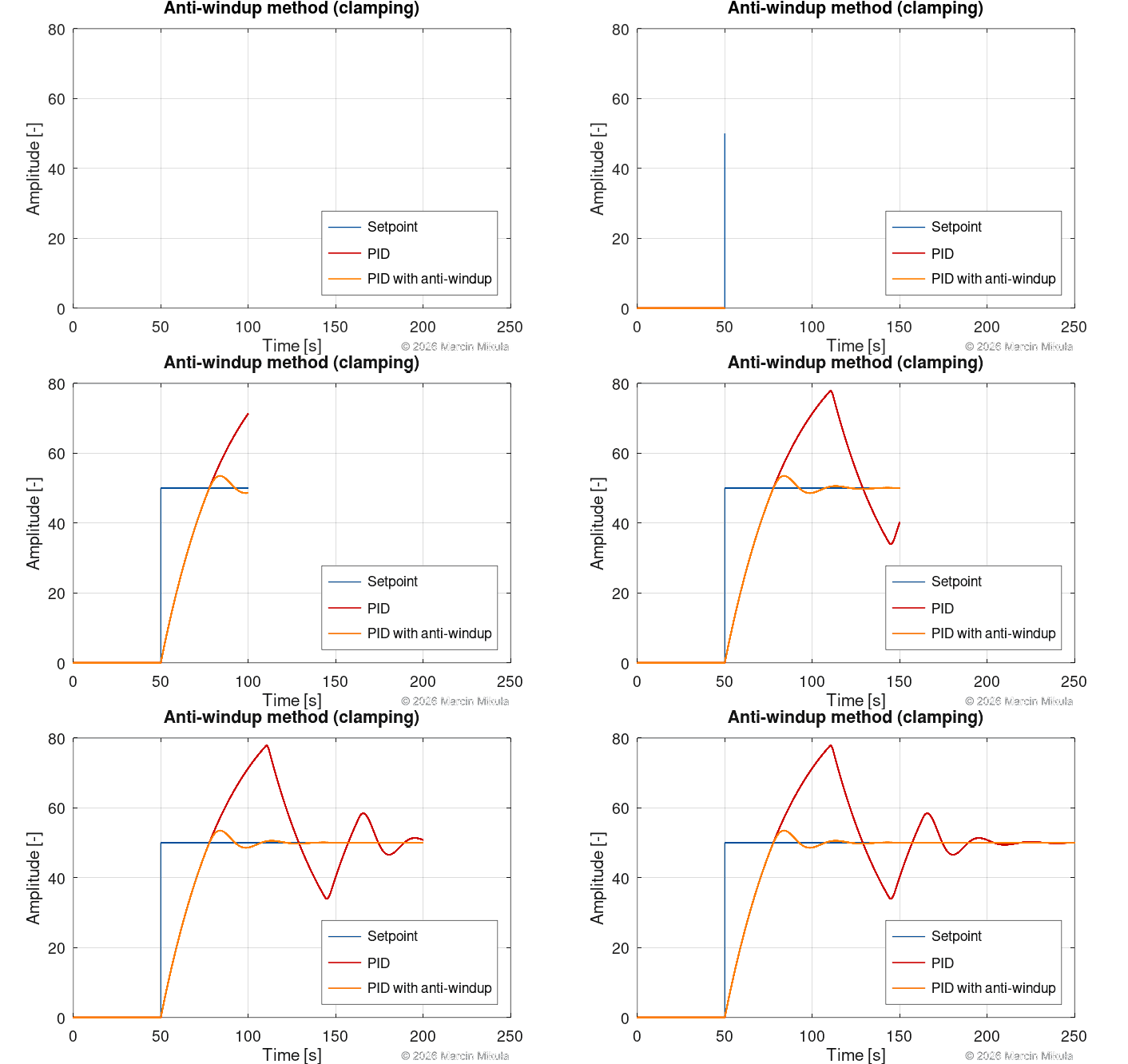
PID response comparison: basic PID vs. PID with anti-windup (clamping).
Clamping - implementation in C on STM32
Although the concept may look complicated, the code is straightforward. The implementation is shown below:
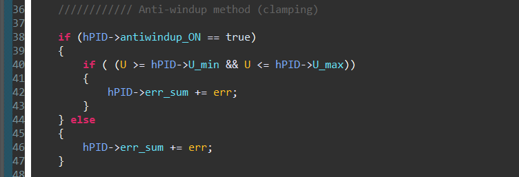
Anti-windup clamping - implementation in embedded C on STM32.
References
- Åström, Karl J., and Tore Hägglund. Advanced PID Control. Triangle Park, NC: International Society of Automation, 2006.
- Brian Douglas - PID Control: A brief introduction
- RS Elektronika - Regulatory PID #158
- Cover photo by Pawel Czerwinski on Unsplash, modified by Marcin Mikuła.